ComplexBandstructure¶

class ComplexBandstructure(configuration, energies=None, k_point=None, energy_zero_parameter=None)¶

Analysis class for calculating the complex bandstructure for a bulk configuration.

Parameters:

configuration (BulkConfiguration) – The bulk configuration with an attached calculator for which to calculate the complex bandstructure.
energies (PhysicalQuantity of type energy) – The energies for which to calculate the complex bandstructure. Note: energies are relative to energy_zero_parameter.
Default: numpy.linspace(-2, 2, 101) * eV
k_point (tuple of floats) – The 2-dimensional fractional k-point (in the kA-kB plane) for which to calculate the complex bandstructure. The k-point is given as a tuple of length 2.
Default: (0, 0)
energy_zero_parameter (FermiLevel | AbsoluteEnergy) – The choice for the energy zero. Note: This also affects the energies parameter.
Default: FermiLevel

energies()¶

Returns:: The energies for which the complex bandstructure is calculated.
Return type:: PhysicalQuantity of type energy

energyZero()¶

Returns:: The energy zero.
Return type:: PhysicalQuantity of type energy

evaluate(spin=None)¶

Method for obtaining the complex bandstructure for a specific spin. The complex bandstructure has two components, propagating modes and decaying modes. Both types of modes can be characterized by a value k. For propagating modes k is real, giving the Bloch phase factor in the reciprocal C-direction, whereas decaying modes have a complex value of k.

Parameters:: spin (Spin.Up | Spin.Down | Spin.All) – The spin to calculate for.
Default: Spin.All
Returns:: A tuple with two lists, the first corresponding to the propagating modes and the second corresponding to the decaying modes. The lists are ordered according to energy and each entry is a PhysicalQuantity with a (1/Angstrom) unit. The lists have different lengths (and can have zero length) corresponding to the number of modes at this energy.
Return type:: tuple of lists

fermiLevel(spin=None)¶

Parameters:: spin (Spin.Up | Spin.Down | Spin.All) – The spin the Fermi level should be returned for. Must be either Spin.Up, Spin.Down, or Spin.All. Only when the band structure is calculated with a fixed spin moment will the Fermi level depend on spin.
Default: Spin.All
Returns:: The Fermi level in absolute energy.
Return type:: PhysicalQuantity of type energy

fermiTemperature()¶

Returns:: The Fermi temperature.
Return type:: PhysicalQuantity of type temperature

kPoint()¶

Returns:: The 2-dimensional fractional k-koint for which the complex bandstructure is calculated.
Return type:: tuple of floats

layerSeparation()¶

Returns:: The distance between layers of the crystal in the transport direction. The transport direction is perpendicular to the AB-plane. This value is called ‘L’ in the GUI.
Return type:: PhysicalQuantity of type length

metatext()¶

Returns:: The metatext of the object or None if no metatext is present.
Return type:: str | None

nlprint(stream=None)¶

Print a string containing an ASCII table useful for plotting the AnalysisSpin object.

Parameters:: stream (python stream) – The stream the table should be written to.
Default: NLPrintLogger()

repetition()¶: Deprecated

setMetatext(metatext)¶

Set a given metatext string on the object.

Parameters:: metatext (str | None) – The metatext string that should be set. A value of “None” can be given to remove the current metatext.

spins()¶

Returns:: The available spin components.
Return type:: tuple of Spin.Up | Spin.Down | Spin.All

uniqueString()¶: Return a unique string representing the state of the object.

Usage Examples¶

Calculate the complex bandstructure of silicon in the (100) direction, using a fast semi-empirical method, and save it to a file:

# Set up a Si (100) minimal configuration
vector_a = [3.84001408591, 0.0, 0.0]*Angstrom
vector_b = [0.0, 3.84001408591, 0.0]*Angstrom
vector_c = [1.92000704296, 1.92000704296, 2.7153]*Angstrom
lattice = UnitCell(vector_a, vector_b, vector_c)

elements = [Silicon, Silicon]

fractional_coordinates = [[  2.50000000e-01,   7.50000000e-01,   5.00000000e-01],
                          [  3.33066907e-16,   2.22044605e-16,   1.00000000e+00]]

bulk_configuration = BulkConfiguration(
    bravais_lattice=lattice,
    elements=elements,
    fractional_coordinates=fractional_coordinates
    )

# Define calculator - fast Slater-Koster method
calculator = SlaterKosterCalculator(
    basis_set=Vogl.Si_Basis,
    numerical_accuracy_parameters=NumericalAccuracyParameters(
                k_point_sampling=(4, 4, 2))
     )
bulk_configuration.setCalculator(calculator)

# Calculate, save, and print the complex band structure
complex_bandstructure = ComplexBandstructure(
    configuration=bulk_configuration,
    energies=numpy.linspace(-2,5,501)*eV,
    k_point=(0,0),
    )
nlsave('si_100_cbs.hdf5', complex_bandstructure)
nlprint(complex_bandstructure)

si_complex_band.py

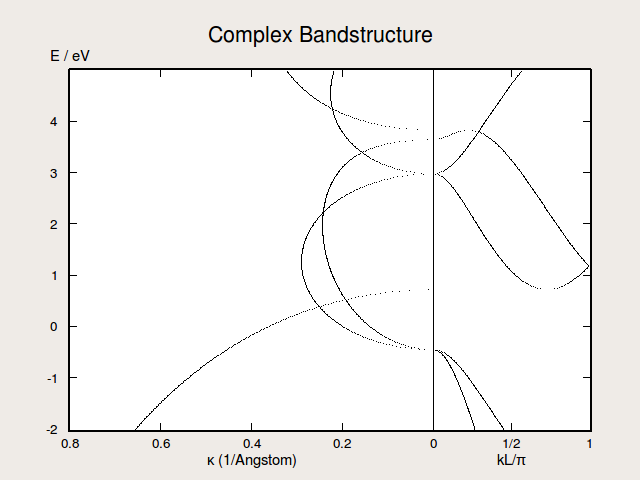
../../../_images/complex_bands.png — Fig. 147 Complex bandstructure for silicon along the (100) direction. The right-hand side of the plots illustrates the real bands while the left-hand side of the plot shows the imaginary part of \(k_C\) for the complex bands.¶

Notes¶

The ComplexBandstructure is calculated for a specified energy, \(E\), and k-point, \(k_A, k_B\), in the plane spanned by the reciprocal A and B vectors. These are provided as input parameters for the calculation. The solutions are the eigenstates, \(\psi_{n {\bf k}}\), of the Schrödinger equation

\[H \psi_{n {\bf k}} = E \psi_{n {\bf k}}\]

with no boundary conditions imposed in the direction perpendicular to the plane spanned by the unit cell vectors \({\bf A}\) and \({\bf B}\). We may write these eigenstates as

\[\psi_{n {\bf k}}({\bf r}) = u_{\bf k}({\bf r}) e^{-i {\bf k}_{AB} {\bf r}_{AB}} e^{-i k_C r_C},\]

where \(u_{\bf k}\) is a periodic function and \(k_C\), in general, is a complex number. The solutions with a purely real \(k_C\) are the usual Bloch states and we thus obtain the normal band structure. The solutions with a complex \(k_C\) form the complex band structure.
The solutions, \(k_C\), can be obtained after the calculation by using the method evaluate(). To print the data, use the method nlprint. In the figure above, which is obtained by plotting the complex band structure in QuantumATK, the k-values for the real band structure are normalized by \(L\) , the layer separation perpendicular to the AB-plane. The value of \(L\) can be extracted by using the method layerSeparation().
The ComplexBandstructure (and the real bands) is computed along the reciprocal C vector, which is perpendicular to the \({\bf A}\) and \({\bf B}\) unit cell vectors. Thus, if the ComplexBandstructure is desired in a particular direction, like (100) as in the example above, the unit cell should be set up such that this direction is perpendicular to the AB-plane. This is most easily achieved by using the Surface tool in the Builder in QuantumATK and choosing a “Periodic (bulk-like)” type of cell with a minimal number of layers.
The implementation of the computation of the complex band structure in QuantumATK follows the method described in Ref. [1].