EffectiveMass
- class EffectiveMass(configuration, symmetry_label=None, kpoint_cartesian=None, kpoint_fractional=None, bands_below_fermi_level=None, bands_above_fermi_level=None, band_index=None, stencil_order=None, delta=None, direction_cartesian=None, direction_fractional=None, method=None)
Constructor for the effective mass object.
- Parameters:
configuration (
BulkConfiguration) – The bulk configuration with an attached calculator for which to calculate the effective mass.symmetry_label (str) – The k-point (as a symmetry point) at which to calculate the effective mass. This option is mutually exclusive to
kpoint_cartesianandkpoint_fractional. Default:'G'(Gamma-point)kpoint_cartesian (PhysicalQuantity of type inverse length) – The k-point (in Cartesian coordinates) at which to calculate the effective mass. This option is mutually exclusive to
symmetry_labelandkpoint_fractional. Default:[0.0, 0.0, 0.0] * Angstrom**-1kpoint_fractional (list(3) of floats) – The k-point (in fractional coordinates) at which to calculate the effective mass. This option is mutually exclusive to kpoint_cartesian and symmetry_label. Default:
[0.0, 0.0, 0.0]bands_below_fermi_level (int) – The number of bands below the Fermi level per principal spin channel to include. This option is mutually exclusive to
band_index. Default:1bands_above_fermi_level (int) – The number of bands above the Fermi level per principal spin channel to include. This option is mutually exclusive to
band_index. Default:1band_index (int) – The band index at which to calculate the effective mass. This option is mutually exclusive to
bands_below_fermi_levelandbands_above_fermi_level.stencil_order (int) – The number of points to use in the second order derivative stencil. Default:
5delta (PhysicalQuantity of type inverse length) – The distance between neighboring points in the stencil. Default:
0.001 * Angstrom**-1direction_cartesian (PhysicalQuantity of type inverse length) – Direction in Cartesian coordinates along which to calculate the effective mass. This option is mutually exclusive to
direction_fractional. Default:[1, 0, 0] * Angstrom**-1direction_fractional (list(3) of floats) – Direction in fractional coordinates along which to calculate the effective mass. This option is mutually exclusive to
direction_cartesian.method (
Numerical|Analytical) – The method for calculating the effective mass. The optionAnalyticalis not supported byPlaneWaveCalculator. Default:Numerical
- energies()
- Returns:
The band energies.
- Return type:
PhysicalQuantity of type energy
- evaluate(spin=None, band=None)
Return the effective mass.
- Parameters:
spin (
Spin.Up|Spin.Down|Spin.All) – The spin for which to evaluate the effective mass. For non-collinear and spin-orbit calculations useSpin.All. Default:Spin.Allband (int) – The band for which to evaluate the effective mass. Default: All bands
- Returns:
The effective mass.
- Return type:
PhysicalQuantity with the unit
electron_mass
- kPoint()
- Returns:
The k-point for which the effective mass was calculated.
- Return type:
numpy.array
- metatext()
- Returns:
The metatext of the object or None if no metatext is present.
- Return type:
str | None
- nlprint(stream=None)
Print a string containing an ASCII table useful for plotting the AnalysisSpin object.
- Parameters:
stream (python stream) – The stream the table should be written to. Default:
NLPrintLogger()
- setMetatext(metatext)
Set a given metatext string on the object.
- Parameters:
metatext (str | None) – The metatext string that should be set. A value of “None” can be given to remove the current metatext.
- uniqueString()
Return a unique string representing the state of the object.
Usage Examples
The effective mass of electrons and holes is related to the local curvature of the electronic band energy, \(E(k)\):
A finite-difference (FD) representation of derivatives of \(E(k)\) is used to compute the effective mass from band structures. The FD approximation for the local derivative of a function \(f(x)\) is basically derived from a Taylor expansion of \(f(x)\) around the central point, \(x\). The n’th derivative is therefore approximated as a sum over function values multiplied by a weight:
The 5-point FD stencil uses function values in the five points \(x\), \(x \pm h\), and \(x \pm 2h\) to approximate the second-order derivative, \(f''(x)\). This is exact up to and including \(O(h^4)\) contributions to the curvature (for \(h<1\)). Beyond that, accuracy improves as the spacing, \(h\), gets smaller.
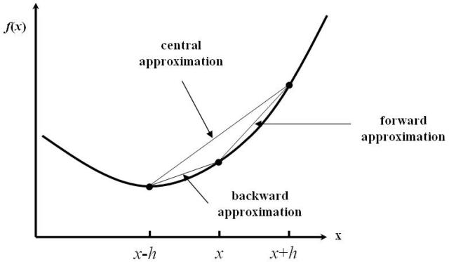
Fig. 153 Finite-difference stencils: Numerical approximations for local derivatives of continuous functions.
The FD method is in general much more accurate than a simple parabolic fit to band energies.
The QuantumATK default is the 5-point FD central stencil with a distance (delta) of 0.001 Å-1
between each point. This gives very accurate results in most cases. The FD accuracy can in
principle be improved by increasing stencil_order and decreasing delta, but the latter
should not be so small that numerical noise starts dominating the error. The figure below shows
the error on computed effective masses for some realistic combinations of stencil_order and
delta. For more information on 5-point stencils, see the relevant Wikipedia entry.
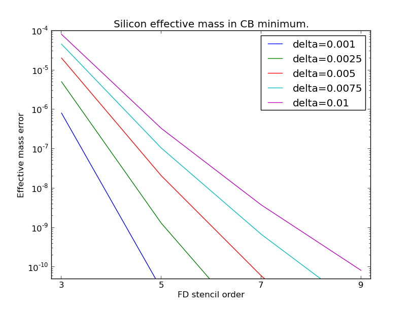
Fig. 154 Errors in the silicon effective mass as a function of the number of points in the FD stencil. Plotted for different distances between the points.
Calculate the effective mass in the silicon conduction band minimum:
# -------------------------------------------------------------
# Bulk configuration
# -------------------------------------------------------------

# Set up lattice
lattice = FaceCenteredCubic(5.4306*Angstrom)

# Define elements
elements = [Silicon, Silicon]

# Define coordinates
fractional_coordinates = [[ 0.  ,  0.  ,  0.  ],
                          [ 0.25,  0.25,  0.25]]

# Set up configuration
bulk_configuration = BulkConfiguration(
    bravais_lattice=lattice,
    elements=elements,
    fractional_coordinates=fractional_coordinates
    )

# -------------------------------------------------------------
# Calculator
# -------------------------------------------------------------
numerical_accuracy_parameters = NumericalAccuracyParameters(
    k_point_sampling=(5, 5, 5),
    density_mesh_cutoff=25.0*Hartree,
    )

calculator = LCAOCalculator(
    numerical_accuracy_parameters=numerical_accuracy_parameters,
    )

bulk_configuration.setCalculator(calculator)
nlprint(bulk_configuration)
bulk_configuration.update()

# -------------------------------------------------------------
# Effective mass
# -------------------------------------------------------------
effective_mass = EffectiveMass(
    configuration=bulk_configuration,
    kpoint_fractional=[0.425000, 0.000000, 0.425000],
    bands_below_fermi_level=1,
    bands_above_fermi_level=1,
    stencil_order=5,
    delta=0.001000*Angstrom**-1,
    )


effective_mass.nlprint()
Notes
Note that the k-points are given in units of the reciprocal vectors \({\bf k}_A\), \({\bf k}_B\), and \({\bf k}_C\). E.g. the symmetry point \(X\) has the fractional k-point coordinates \((\frac{1}{2}, 0, \frac{1}{2})\) since it is described by \(X = \frac{1}{2}{\bf k}_A + \frac{1}{2}{\bf k}_C\). The k-point used in the calculations is thus close to the X-point, where the conduction band has its minimum.
For each band index, three masses are written in the output. The three masses are the eigenvalues of the effective mass tensor given by \([M^{-1}]_{ij} = \hbar^{-2}\frac{\partial^2E(k)}{\partial k_i\partial k_j}\).
In the example above, the three masses of the lowest conduction band are \(m^* = (0.19, 0.19, 0.9)m_e\), in good agreement with experimental values.
For
bands_above_fermi_levelset to a valid integer, \(N_{\text{ba}}\), the total number of bands above the Fermi level will be \(N_{\text{ba}}\) for the spin type unpolarized, and \(2 N_{\text{ba}}\) for polarized and noncollinear. This is because there is only one spin channel in the former case and two spin channels in the latter two cases. Spin-orbit calculations are categorized as non-collinear calculations and therefore follow the same band selection as noncollinear. The same behavior applies for the relation betweenbands_below_fermi_leveland the total number of bands below the Fermi level. The case wherebands_above_fermi_levelis 2 andbands_below_fermi_levelis 1, are illustrated in Fig. 155.
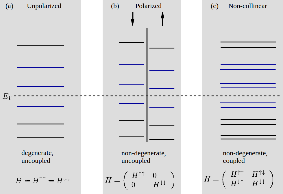
Fig. 155 The total number of bands selected (blue lines) by specifying 2 bands above the Fermi level and 1 band below the Fermi level for (a) an unpolarized, (b) a polarized, and (c) a non-collinear calculation. The Fermi level \(E_{\text{F}}\) is shown as a horizontal dashed gray line. The vertical separation line in (b) signifies that the bands can be categorized according to spin up or down since there is no coupling. The structure of the Hamiltonian for each of the 3 spin types is shown at the bottom.