Adding, Combining, and Modifying Classical Potentials

PDF version

Introduction

The new ATK-ForceField package provides a lot of pre-defined classical potentials covering a broad range of elements and systems. However, if you are interested in a particular potential, which is not yet part of this pre-defined set, you can easily add these parameters and create your own potential, as long as the underlying potential functions are supported. You can also modify single parameters of existing potentials in order to tune the potential to a special reference system. Furthermore, you can combine different potentials to cover a broader range of elements. This tutorial provides a brief overview over this functionality of ATK-ForceField.

Note

For QuantumATK-versions older than 2017, the ATK-ForceField calculator can be found under the name ATK-Classical.

For a detailed overview and documentation of the available potential classes and functions in ATK-ForceField and the underlying TremoloX package, take a look at the TremoloX section of the ATK Reference Manual. There you will find definitions for all functions along with the corresponding parameters.

Note

Be aware that you should always read the underlying publication carefully, if you use a new potential, to ensure that the potential is suited for your desired application.

If possible, you should compare some benchmark values obtained with the classical potential to corresponding experimental values or the results of suitable higher-level calculations, e.g. DFT simulations. This holds in particular for the combination of different potentials, as they might have been parameterized in a certain context and they are not always guaranteed to work in entirely different environments.

Adding a New Classical Potential from Scratch

In this section, you will learn how to add a new parameter set, taken from a potential in the literature, to the ATK-ForceField calculator. You will be guided through the complete setup of a potential from scratch to explain the various contents of a TremoloX potential set. In practice, it is often more convenient to start from a similar potential, send it to the Editor with Script details set to “Show defaults” to report all details of the potential, and then merely edit the parameters in the Editor.

As a first example, you will consider a simple titanium oxide crystal. One of the most popular classical potentials for titania is the one proposed by Matsui and Akaogi (MA) [1], as it reproduces the essential properties of both crystal and amorphous titania systems quite well. Later on, you will set up a potential designed for the simulation of amorphous oxide systems [2].

Setting up the System

To set up a suitable test system, open the Builder, click Add ‣ From database, search for “TiO2”, and select and add the Rutile crystal structure.

You can now send the configuration to the ScriptGenerator to set up the desired optimization, molecular dynamics, or analysis script. For now, you can select any arbitrary calculator as a place holder. A typical simulation script could consist of Calculator, Optimization ‣ OptimizeGeometry, and Analysis ‣ ElasticConstants blocks. For accurate results, set the maximum force and maximum stress values in the OptimizeGeometry settings and the maximum force value in the ElasticConstants settings to 0.001 eV/Å (respectively eV/ų). Furthermore, disable the Constrain cell checkbox in the OptimizeGeometry widget to optimize the cell parameters as well.

Send the script to the Editor.

Setting up the Potential

In the Editor, locate the block where the potential is defined (i.e. everything after the BulkConfiguration and before the OptimizeGeometry block) and delete it.

To define a new TremoloX potential you first need to initialize a new TremoloXPotentialSet object. You can do this by adding the following line:

potentialSet = TremoloXPotentialSet('MatsuiAkaogi_TiO')

The string in parethesis defines the name of the potential, but it does not have any influence on its functionality.

As the potential set is currently empty, you need to add all necessary components. You should start with adding the ParticleType. In this case, add one titanium and one oxygen particle type by inserting these two lines into the script:

potentialSet.addParticleType(ParticleType(symbol='O', mass=15.9994*atomic_mass_unit, charge=-1.098))
potentialSet.addParticleType(ParticleType(symbol='Ti', mass=47.867*atomic_mass_unit, charge=2.196))

The partial charges are taken from Ref. [1]. The MA potential consists of two interaction types:

1. A Tosi-Fumi (often also called Buckingham) type potential (i.e. a combination of an exponential, repulsive contribution and an attractive van der Waals part)

2. Electrostatic coulomb interactions, which model the partial ionization of the atoms.

The first part can be added by using the TosiFumiPotential, which implements the potential function

\[V(r) = A e^{B(\sigma -r)} - \frac{C}{r^6} - \frac{D}{r^8} \, .\]

If you compare this form to the equation given in Ref. [1], you will notice that the last term is not required, implying that D must be set to zero. Take care with the energy unit in Ref. [1], which is kJ/mol. The parameters must be given in that unit or converted to electron volt. The A, B, C, D, and \(\sigma\) parameters can be set as follows:

potentialSet.addPotential(TosiFumiPotential(particleType1='O',
                                            particleType2='Ti',
                                            A=0.811696*kiloJoulePerMol,
                                            B=5.154639*Angstrom**-1,
                                            sigma=2.8171*Angstrom,
                                            C=1215.0*kiloJoulePerMol*Angstrom**6,
                                            D=0.0*eV*Angstrom**8,
                                            r_i=6.0*Angstrom,
                                            r_cut=7.5*Angstrom))
potentialSet.addPotential(TosiFumiPotential(particleType1='O',
                                            particleType2='O',
                                            A=0.979056*kiloJoulePerMol,
                                            B=4.27350*Angstrom**-1,
                                            sigma=3.2678*Angstrom,
                                            C=2916.0*kiloJoulePerMol*Angstrom**6,
                                            D=0.0*eV*Angstrom**8,
                                            r_i=6.0*Angstrom,
                                            r_cut=7.5*Angstrom))
potentialSet.addPotential(TosiFumiPotential(particleType1='Ti',
                                            particleType2='Ti',
                                            A=0.644336*kiloJoulePerMol,
                                            B=6.49351*Angstrom**-1,
                                            sigma=2.3664*Angstrom,
                                            C=506.25*kiloJoulePerMol*Angstrom**6,
                                            D=0.0*eV*Angstrom**8,
                                            r_i=6.0*Angstrom,
                                            r_cut=7.5*Angstrom))

The first two arguments in each potential determine which two particle types the potential is supposed to act between. The additional parameters r_*i* and r_cut determine the range and cutoff behavior. In this case, the potential follows the original form for distances below 6 Å, whereas for larger distances a smoothing function is invoked for ranges up to 7.5 Å. At larger distances these interactions are assumed to be zero.

The electrostatic interactions are taken into account by adding a suitable Coulomb solver. All Coulomb solvers use the partial charges that you have defined for the particle types. The default algorithm in ATK-ForceField is CoulombDSF employing a cutoff and a damped shifted force (DSF) to smooth the transition [2]. To achieve a high precision with this method (which can be important particularly for static calculations, such as elastic constants, phonons, or lattice constants) the cutoff has to be chosen sufficiently high (e.g. ≥ 15 Å). Here, we will instead use the smooth-particle-mesh-Ewald method (CoulombSPME), which automatically takes care of the long-ranged contributions of the Coulomb interactions. This Coulomb solver is added via the line:

potentialSet.setCoulombSolver(CoulombSPME(r_cut=9.0*Angstrom))

Finally, you have to initialize the actual TremoloXCalculator and pass the created potential set as argument. Following that, you have to attach the calculator to the bulk configuration:

calculator = TremoloXCalculator(parameters=potentialSet)
bulk_configuration.setCalculator(calculator)

The remaining part of the script can be left as it is. An example script can be found in the file TiO2_Matsui.py.

Now, you can send the script to the JobManager and start the calculation. The results should be consistent with Ref. [1].

A Potential for Amorphous Oxides

In this example, another potential is introduced, which is designed to simulate amorphous materials, such as titanium, silicon, hafnium, or tantalum oxide, as well as their mixed oxides [3].

Note

From QuantumATK 2015 on, this potential is already available as the pre-defined potential Trinastic_HfOSiTaTi_2013.

To test the potential, you can, for instance, use the rutile configuration from the previous example. The potential is similar to the MA potential, shown above, but additionally it includes a MorsePotential.

\[V(r) = E_{ij} \left [ \left(1 - e^{-k_{ij}(r-r_0)} \right)^2 - 1 \right ]\]

In fact, the formula presented in Ref. [3] omits the the last contribution in the squared brackets. However, as this term only represents a constant offset in the energy, it has no influence on the forces in an MD simulation, and we shall therefore neglect this discrepancy here. Although the potential terms could in principle be set up similar to the previous example by using the TosiFumiPotential, we will present an alternative approach by adding all terms individually.

To obtain the potential, you need an exponential repulsive contribution, which will be taken from the BuckinghamPotential, a dispersion term, for which you will use a LennardJonesMNPotential, and finally a MorsePotential.

The potential set up is demonstrated for the example of the Ti-O interactions. The other elements follow the same scheme by inserting the corresponding element-pair-specific potential parameters from Ref. [3].

Start by initializing a new TremoloXPotentialSet and adding the particle types with the corresponding partial charges:

potential_set = TremoloXPotentialSet('Trinastic_JCP2013')
potential_set.addParticleType(ParticleType(symbol='O', mass=15.9994*atomic_mass_unit, charge=-1.2))
potential_set.addParticleType(ParticleType(symbol='Ti', mass=47.867*atomic_mass_unit, charge=2.4))

Then define the repulsive Buckingham term:

potential_set.addPotential(BuckinghamPotential(particleType1='O',
                                               particleType2='Ti',
                                               A=5105.12*eV,
                                               rho=0.2253*Angstrom,
                                               r_i=6.0*Angstrom,
                                               r_cut=7.5*Angstrom))

Add the dispersion term. You will only need the attractive part of the Lennard-Jones potential, i.e. the A-parameter has to be set to zero:

potential_set.addPotential(LennardJonesMNPotential(particleType1='O',
                                                   particleType2='Ti',
                                                   A=0.0*eV*Angstrom**12,
                                                   B=20.0*eV*Angstrom**6,
                                                   m=12,
                                                   n=6,
                                                   r_cut=10.0*Angstrom))

Add the Morse potential:

potential_set.addPotential(MorsePotential(particleType1='O',
                                          particleType2='Ti',
                                          E_0=0.3478*eV,
                                          k=1.9*Angstrom**-1,
                                          r_0=1.96*Angstrom,
                                          r_i=6.5*Angstrom,
                                          r_cut=7.0*Angstrom))

Finally, set up a Coulomb solver, e.g. CoulombSPME or CoulombDSF to calculate the electrostatic interactions, and initialize a new TremoloXCalculator with this potential set:

potential_set.setCoulombSolver(CoulombSPME(r_cut=9.0*Angstrom))
calculator = TremoloXCalculator(parameters=potential_set)

In Ref. [3], an alternative strong parameterization is proposed, which can be implemented by inserting the corresponding parameters instead of the ones shown above. The implementation of the interactions between the remaining element pairs works similarly. From the parameter table in Ref. [3], you will find that for some element combinations the Morse energy parameter is zero, which means that no Morse potential is required between these elements.The full potential can be found in the file script_Trinastic_potential.py.txt.

Combining a Tersoff and a Lennard-Jones Potential

In this section, you will learn how you can combine Tersoff and Lennard-Jones (LJ) potentials, to simulate a single lithium atom in a graphite cell. This combination of materials is particularly interesting, as it provides a very simple model of a typical anode in lithium ion batteries. The combination of Tersoff and LJ-potentials is typically used for multi-component materials where the individual components interact only weakly with each other, predominantly via repulsive and van der Waals forces. The strong bonded interaction within a component, in this example graphite, can then be described by a Tersoff potential, or another suitable potential for that material.

In this example, you will adopt the parameters of Ref. [4]. Be aware that they have not been tested extensively for this system. Therefore, they should only be considered a starting point for your own investigations.

Setting up the System

To set up a test system, open the Builder and add a graphite cell via Add ‣ From database. Increase the size of the cell by clicking Bulk tools ‣ Repeat, and make a 4x4x2 repetition of the unit cell.

Select a triangle of 3 atoms (one in the second layer, two in the third layer) as shown in the picture.

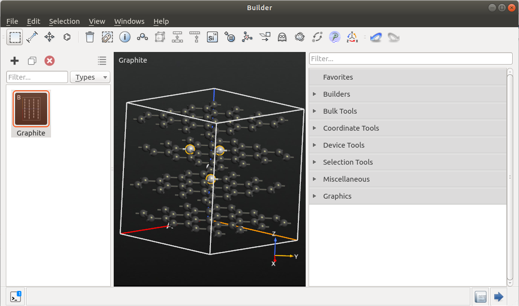
Place an additional atom in the center of the selected atoms, by clicking on the icon in the toolbar (see picture). This atom will later be converted into lithium, but for now we will retain it as carbon.

Send the configuration to the ScriptGenerator using the button. In the ScriptGenerator, add a Calculators ‣ ForceFieldCalculator object, and then the simulation task of your choice, e.g. an Optimization ‣ MolecularDynamics block. Open the ForceFieldCalculator settings, and select the Tersoff_C_2005 potential (this will be the base potential for the graphite). Under Results, select “Do not save” and uncheck Print results to summary log. In the Output Settings, set Script Detail to “Show defaults”, and send the script to the Editor.

At first, locate the element list. Change the name of the last element in the list from Carbon to Lithium. (If you had done this already in the Builder, it would not have been possible to select the Tersoff potential in the ScriptGenerator, since it doesn’t support lithium.)

If you now take a look at the calculator section, you will find the detailed definition of the Tersoff potential. This is due to the Show defaults option. Locate the line where the ‘C’ element definition is added via the addParticleType() method. Make a copy (to invoke two addParticleType() calls), and modify the relevant lines as shown below:

potentialSet.addParticleType(ParticleType(symbol='C',
                                          mass=12.0107*atomic_mass_unit,
                                          charge=None,
                                          # Sigma and epsilon from Ref [3].
                                          sigma=3.3611*Ang,
                                          epsilon=0.004207*eV))
potentialSet.addParticleType(ParticleType(symbol='Li',
                                          mass=6.941*atomic_mass_unit,
                                          charge=None,
                                          # Sigma and epsilon from Ref [3].
                                          sigma=0.826*Ang,
                                          epsilon=0.271115*eV))

For carbon, the LJ-parameters epsilon and sigma have been added and set to the values taken from Ref [4]. For lithium, you first have to change the symbol and the atomic mass and then set the corresponding LJ-parameters. Note that in this case, we consider neutral lithium atoms, i.e. without defining a partial charge, as this is the preferred state in the anode (in contrast to lithium ions in the cathode).

The LJ-potential does not become active by specifying the particle parameters alone. You additionally have to add the corresponding potential function. To this aim, add the following two lines:

potentialSet.addPotential(LennardJonesPotential(particleType1='C',
                                                particleType2='Li',
                                                r_cut=9.0*Ang))
potentialSet.addPotential(LennardJonesPotential(particleType1='Li',
                                                particleType2='Li',
                                                r_cut=9.0*Ang))

This will add LJ-potentials between carbon and lithium, as well as between lithium and lithium. Note that there is no LJ-potential between carbon atoms, as these interactions are sufficiently defined by the Tersoff-potential (the LJ would just be a tiny correction).

The Lennard-Jones potential in ATK-ForceField is defined as

\[V_{ij}(r) = 4\epsilon_{ij} \left [ \left(\frac{\sigma_{ij}}{r} \right)^{12} - \left(\frac{\sigma_{ij}}{r} \right)^{6} \right]\]

and uses the combination rules to obtain \(\sigma_{ij}\) and \(\epsilon_{ij}\) parameters between different elements that you can find in the LennardJonesSplinePotential documentation page.

You should always check whether the combination rules recommended for the chosen LJ-parameters agree with this definition. If not, you should use the more general LennardJonesMNPotential.

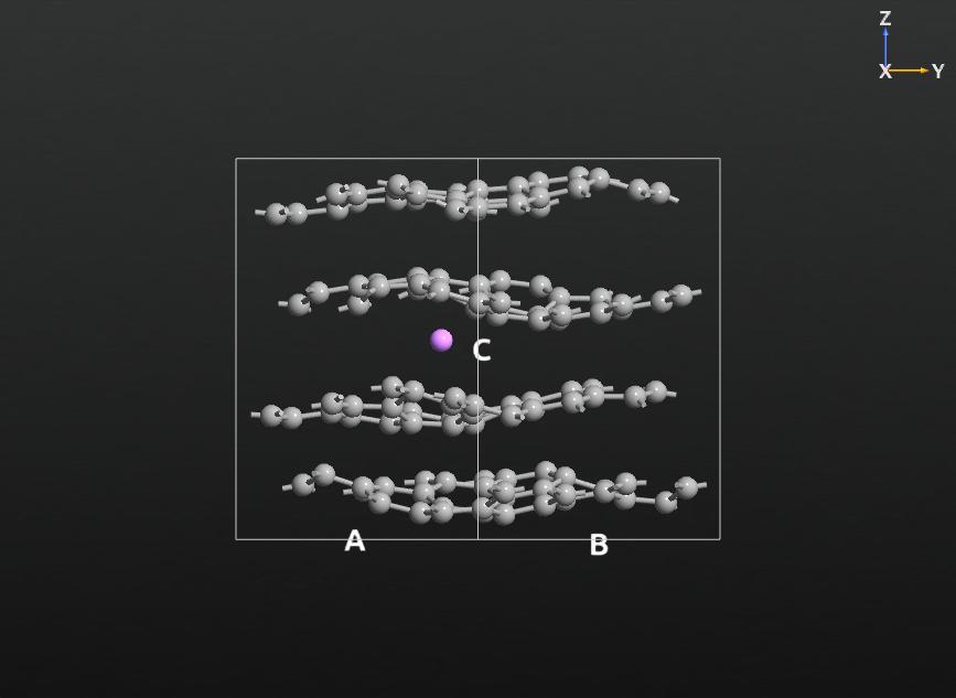
An example of the final script can be found in Script_graphite_lithium.py. You can add any optimization, molecular dynamics, or analysis block, compatible with ATK-ForceField. This picture shows a snapshot of an MD simulation of the lithium-graphite system.

Intra- and Inter-Layer Cohesion in MoS₂

Note

If you are using QuantumATK 2014, you should make sure that you have ugraded to QuantumATK 2014.3 (or later) to run this part of the tutorial, as earlier versions may cause some problems.

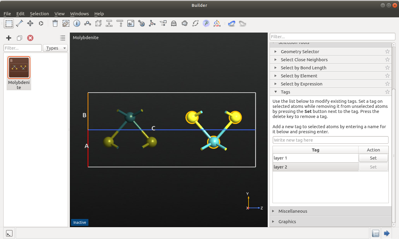
In this last example you will learn how to define a potential only on the selected atoms, using tags. We consider a molybdenite (MoS₂) crystal where the intralayer interactions are described by a Stillinger-Weber potential, while the comparably weaker inter-layer interactions are again modelled by a Lennard-Jones potential, as described in Ref. [4].

To set up the system, open the Builder and search for and add the molybdenite structure from the database. Select one layer by drawing a rectangle around it and add a tag with the name “layer1” (via Selection Tools ‣ Tags). Repeat the procedure for the second layer, using the name “layer2”.

Send the configuration to the ScriptGenerator.

In the ScriptGenerator add a Calculators ‣ ForceFieldCalculator and an Optimization ‣ OptimizeGeometry block. Open the ATK-ForceField calculator and select the StillingerWeber_MoS_2013 potential. Under Results, select “Do not save” and close the widget. Open the OptimizeGeometry widget and adjust the setting for a geometry and stress optimization, as described in the first example.

Send the final script to the Editor.

In the python-script, locate the line where the Stillinger-Weber-potential is defined. Copy the line, and adjust both lines in the following way:

sw_layer1 = StillingerWeber_MoS_2013(tags='layer1')
sw_layer2 = StillingerWeber_MoS_2013(tags='layer2')

This will define each potential only between the atoms belonging to the corresponding tagged group. Furthermore, you have to define a Lennard-Jones potential, which acts only between the sulfur atoms of different groups. This can be done by adding the following lines of code:

# Define a new potential for the interlayer interaction.
lj_interlayer_potential = TremoloXPotentialSet(name="InterLayerPotential")
# Add particle type definitions for both types.
lj_interlayer_potential.addParticleType(ParticleType.fromElement(Molybdenum))
lj_interlayer_potential.addParticleType(ParticleType.fromElement(Sulfur, sigma=3.13*Angstrom, epsilon=0.00693*eV))
# Add Lennard-Jones potentials between the sulfur atoms of different layers.
lj_interlayer_potential.addPotential(LennardJonesPotential('S', 'S', r_cut=10.0 * Angstrom))
lj_interlayer_potential.setTags(['layer1', 'layer2'])

The Lennard-Jones parameters are taken from Ref. [5]. The last line ensures that the Lennard-Jones-potential only acts between alternating layers.

Finally, all three potential sets have to be combined in the TremoloX-calculator. To accomplish this, add the following lines:

# Combine all 3 potential sets in a single calculator.
calculator = TremoloXCalculator(parameters=[sw_layer1, sw_layer2, lj_interlayer_potential])

After defining the potential, the script continues as usual, by adding the calculator to the bulk configuration and performing the geometry optimization. The final script can be found in the file Molybdenite_SW_plus_LJ.py for comparison.

If you run the script, you will obtain optimized lattice constants, which should be very similar to the ones reported in Ref. [5].

References

[1] (1,2,3,4,5)

M Matsui and M. Akaogi: Molecular dynamics simulations of the structural and physical properties of the four polymorphs of TiO2. Mol. Sim. 6, 239 (1991)

[2] (1,2)

C.J. Fennell and J.D. Gezelter: Is the Ewald summation still necessary? Pairwise alternatives to the accepted standard for long-range electrostatics. J. Chem. Phys. 124, 234104 (2006)

[3] (1,2,3,4,5)

J.P. Trinastic, R. Hamdan, Y. Wu, L. Zhang, H.-P. Cheng: Unified interatomic potential and enery barrier distributions for amorphous oxides. J. Chem. Phys. 139, 154506 (2013)

[4] (1,2,3)

O. N. Kalugin, V. V. Chaban, O. V. Prezhdo: Microscopic Structure and Dynamics of Molecular Liquids and Electrolyte Solutions Confined by Carbon NanoTubes: Molecular Dynamics Simulations. Carbon Nanotubes - Synthesis, Characterization, Applications (2011), Siva Yellampalli (Ed.).

[5] (1,2)

J.-W. Jiang, H.S. Park, T. Rabczuk: Molecular dynamics simulations of single-layer molybdenum disulphide (MoS₂): Stillinger-Weber parameterization, mechanical properties and thermal conductivity J. Appl. Phys. 114, 064307 (2013)