Bulk Magnetic Anisotropy Energy

Version: S-2021.06

Downloads & Links

PDF version
FePt.py
FePt-SO-SCF-loop-over-angles.py
plot-E-vs-theta-FT-and-SO-Etot.py
MagneticAnisotropyEnergy
Basic QuantumATK Tutorial
ATK Reference Manual

In this tutorial you will learn how to use the MagneticAnisotropyEnergy study object to calculate the magneto-crystalline anisotropy (MCA) energy of bulk FePt in the \(L1_0\) phase.

The result of the MagneticAnisotropyEnergy will be compared with self-consistent total energy calculations including spin-orbit coupling, and you will learn about the most important numerical parameters to converge, when performing MCA calculations.

Introduction

The magnetic anisotropy energy (MAE) is the energy difference between two magnetization directions. Different physical mechanisms can contribute to the MAE, but here we are concerned with the magnetocrystalline anisotropy (MCA). Another important contribution is the shape-anisotropy, which occurs if the magnetic material has a non-spherical shape.

The origin of the MCA is the spin-orbit coupling and it is characterized by the dependence of the energy of a magnetic system on the orientation of the magnetization with respect to the crystallographic structure of the material. The axis (or plane) corresponding to the minimum of energy is the so-called easy axis (plane).

The MAE is of central interest for both fundamental and practical reasons, with STT-MRAM being one of the most important technological examples.

STT-MRAM

Spin-transfer torque magnetic random access memory (STT-MRAM) enables higher densities, low power consumption and reduced cost compared to regular MRAM devices. The main advantage of STT-MRAM over regular MRAM is the ability to scale the STT-MRAM chips to achieve higher densities at a lower cost.

One of the key requirements of an STT-MRAM device is of course to be able to store information. This requires that the energy-barrier between the ‘1’ and ‘0’ states is large enough to not allow switching due to thermal fluctuations. The MCA is a key element in determining the energy barrier and thus the thermal stability of a STT-MRAM memory unit.

Theory

The magnetic anisotropy energy is defined as the energy difference between two spin orientations:

\[MAE = E(\theta_1, \phi_1) - E(\theta_0, \phi_0),\]

where the spin orientation is described by the two spherical angles \(\theta\) and \(\phi\). The MAE can be calculated directly from self-consistent calculations including spin-orbit coupling. This can, however, be computationally quite demanding since spin-orbit calculations can some-times be difficult to converge at the desired accuracy.

Force theorem

In the MagneticAnisotropyEnergy study object we calculate the MAE using the force theorem, which allows you to evaluate the energy difference using non-self consistent band energies [1]:

\[MAE = \sum_i f_i(\theta_1, \phi_1) \epsilon_i(\theta_1, \phi_1) - \sum_i f_i(\theta_0, \phi_0) \epsilon_i(\theta_0, \phi_0),\]

where \(f_i(\theta, \phi)\) is the occupation factor for band i (including both band and k-point index) with the spin orientation \((\theta, \phi)\) and \(\epsilon_i(\theta, \phi)\) is the corresponding band energy.

The use of the force theorem (FT) has been validated in several papers, e.g. [2], [3] against self-consistent calculations of total energies. Using the FT has several advantages over the self-consistent approach:

• It is usually faster since the self-consistent solution of the spin-orbit calculation is computationally significantly more demanding than the polarized one.

• Often it is harder to achieve good convergence for a spin-orbit calculation than for a polarized one.

• Using the FT approach allows for projection analysis since each band energy has an associated eigenvector that can be projected onto atomic sites or individual orbitals (see the :ref:´mae_bulk_analyze_results´ section). The projection analysis is often helpful in understanding the physics behind the calculated MAE. An example could be the difference between surface/interface atoms and bulk atoms in the contribution to the MAE in a metallic slab [4].

Note

About the naming: In this tutorial, the name magnetic anisotropy energy (MAE) will be used somewhat interchangeably with the name magnetocrystalline anisotropy (MCA). A third name, which is often used, is perpendicular magnetic anisotropy (PMA) and refers to an interface plane, often with a magnetic tunnel junction in mind - see also Magnetic Anisotropy Energy of Fe-MgO-Fe MTJ structure. In the literature, the MAE will sometimes include the so-called shape anisotropy as well, which accounts for the (classical) dipole-dipole interaction between magnetic moments [1].

MAE of FePt

\(L1_0\) FePt has been studied in a number of scientific papers and is one of the materials with the largest known MCA. In this tutorial we will use the structure from [3]. It is well-known that even small structural difference can have a big impact on the MCA. In order to have a direct comparison to the calculated values in [3] we will not perform any structural relaxation.

Structure

The structure of the FePt cell is shown below.

# -------------------------------------------------------------
# Bulk Configuration
# -------------------------------------------------------------

# Set up lattice
lattice = SimpleTetragonal(2.722*Angstrom, 3.71281*Angstrom)

# Define elements
elements = [Platinum, Iron]

# Define coordinates
fractional_coordinates = [[ 0.5,  0.5,  0.5],
                          [ 0. ,  0. ,  0. ]]

# Set up configuration
bulk_configuration = BulkConfiguration(
    bravais_lattice=lattice,
    elements=elements,
    fractional_coordinates=fractional_coordinates
    )

Copy the python script with the bulk configuration and paste it into the Builder:

1. Press the Add icon

2. Select From Clipboard

3. Press F2 and rename the structure to FePt.

The structure should look like this:

Send the structure to the Script Generator using the icon.

Setup MagneticAnisotropyEnergy calculation

MCA values are small quantities, most often below 1 meV/atom. This puts strong requirements on the numerical settings and a careful convergence study is recommended for any use of MagneticAnisotropyEnergy.

In the Convergence of results section we will go into more details about convergence studies. For now we will setup a calculator with reasonably well-converged settings resulting in calculated MCA values converged within \(\sim 0.2\) meV.

In the Script Generator add an LCAOCalculator. Open the calculator block and apply the following changes (see image below):

• Change the Spin to Noncollinear Spin-Orbit

• Change the Broadening to 300 K

• Finally increase the k-point density to 7 Å (select from the Preset Densities combo box)

Close the calculator widget and add a MagneticAnisotropyEnergy block, located under the Study object category. Open the MagneticAnisotropyEnergy block to change the settings (see image below):

• Increase the number of Theta angle points to 7.

If you are only interested in the energy difference between the out-of plane, \(\theta=0\), and in-plane, \(\theta=90\), configurations it suffice to just have two Theta angle points. For tutorial purposes we add more angles to inspect the behavior of \(MAE(\theta)\).

• Increase the k-point density to 17 Å (select from the Preset densities combo box)

• Leave the Projections to Sites, but notice that you can also project on Sites and Shells or Sites and Orbitals. These options can be useful for analysis of the MAE at e.g. interfaces, and will be addressed in a different tutorial.

Close the MagneticAnisotropyEnergy widget. You are now ready to submit the calculations. Note that due to the rather high k-point sampling in both the LCAOCalculator and in the MagneticAnisotropyEnergy object, the calculation is somewhat computationally demanding and should preferably be run with several MPI processes.

Send the calculation to the Job Manager using the icon and run the calculation. The calculation can take up to several hours, depending on the available computational resources. On a single node with 24 cores, it takes around 10 minutes with QuantumATK R-2020.09-SP1.

Note

A MagneticAnisotropyEnergy object can only be calculated when the calculator has Spin set to Noncollinear Spin-Orbit.

Analyze results

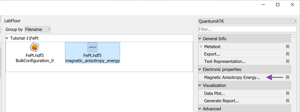
Once the calculation is done, we can inspect the result by either using Text Representation or the dedicated MAE Analyzer:

• Find the Text Representation button in the right-hand panel. This will show a summary of the calculations as shown here:

# Title: FePt.hdf5 - magnetic_anisotropy_energy
# Type:  MagneticAnisotropyEnergy
+------------------------------------------------------------------------------+
| MagneticAnisotropyEnergy Report                                              |
+------------------------------------------------------------------------------+
+------------------------------------------------------------------------------+
| Calculated angles (Degrees)                                                  |
+------------------------------------------------------------------------------+
| (theta, phi) = (   0.00,    0.00)                                            |
| (theta, phi) = (  15.00,    0.00)                                            |
| (theta, phi) = (  30.00,    0.00)                                            |
| (theta, phi) = (  45.00,    0.00)                                            |
| (theta, phi) = (  60.00,    0.00)                                            |
| (theta, phi) = (  75.00,    0.00)                                            |
| (theta, phi) = (  90.00,    0.00)                                            |
|                                                                              |
+------------------------------------------------------------------------------+
| Total magnetic anisotropy energy (MAE)                                       |
+------------------------------------------------------------------------------+
| MAE = E(theta_1,   phi_1) - E(theta_0,   phi_0)                              |
| MAE = E(  90.00,    0.00) - E(   0.00,    0.00)                              |
| MAE =  2.3823 meV                                                            |
+------------------------------------------------------------------------------+

The bottom of the output shows the final MAE calculated as the energy difference between the first and last angles. The positive MAE value means that the \(\theta=0^\circ\) spin direction has a a lower energy than the \(\theta=90^\circ\) direction.

The calculated MCA values of 2.3 meV is slightly smaller than the values reported in [3] ranging from 2.59 meV for self-consistent total energies calculated with VASP to 2.93 meV calculated with Siesta. As will be shown in Convergence of results, the results ontained so far are not completely converged with respect to k-point sampling. Using higher k-point sampling, the QuantumATK values are 2.5 meV and are thus in very close agreement with the self-consistent results of VASP.

• The result of a MagneticAnisotropyEnergy calculation can also be analyzed with the Magnetic Anisotropy Energy analyzer. Mark the calculated MagneticAnisotropyEnergy on the LabFloor and open the analyzer.

The analyzer shows the contribution to the MAE from different projections, in this case for each atom. It shows the Fe and Pt atoms contribute more or less equally to the total MAE.

The calculated angles can be selected in the Angles combo boxes. Selecting \(\theta_0=0\) and \(\theta_1=90\) will result in the largest values.

In the lower left, the total MAE is shown in units of meV. Just below is shown the K1 value, which here is defined as \(K1 = MAE/(2\cdot A)\) where \(A\) is the cross section area. This quantity is mainly relevant when studying interfaces, where K1 is the surface anisotropy energy density. More details about this can be found in the tutorial Magnetic Anisotropy Energy of Fe-MgO-Fe MTJ structure.

MCA vs. angle

The dependence of the MCA value on the \(\theta\) angle can be shown with a small python script.

import pylab

filename = 'FePt.hdf5'

# Load the MAE object
magnetic_anisotropy_energy = nlread(filename, MagneticAnisotropyEnergy)[0]

# Get the calculated angles
theta_angles = magnetic_anisotropy_energy.thetaAngles()

# Get the calculated MAE values
mae_values = [magnetic_anisotropy_energy.magneticAnisotropyEnergy(
    theta_0=0*Degrees, theta_1=theta).inUnitsOf(meV)
    for theta in theta_angles]

# Get the total MAE
k = mae_values[-1]

# Plot the results
pylab.figure()
pylab.plot(theta_angles, mae_values, 'ko', label='MAE study object')
pylab.plot(theta_angles, k*numpy.sin(theta_angles)**2, 'k-', label='$k\\cdot sin^2(\\theta)$')
pylab.xlabel('$\\theta$  (Deg.)')
pylab.ylabel('MAE  (meV)')
pylab.legend(loc=0)
pylab.show()

Run the script to produce the figure below. In the script, the MAE values are extracted for different theta angles and plotted. The plot shows that the MAE follows a \(k\cdot\sin^2(\theta)\) dependence in agreement with several previous studies, where \(k\) is the maximum MCA (MAE) value.

TotalEnergy calculations

As mentioned above, the MAE calculated with the MagneticAnisotropyEnergy study object is calculated using the force theorem (FT), where the spin-orbit calculation is performed non-self-consistently from a polarized calculation.

It is also possible to directly calculate the MAE from total energy differences of self-consistent spin-orbit calculation as will be shown below. It can often speedup the calculation by first performing a relatively inexpensive spin-polarized calculation and use this as an initial state for the more expensive Noncollinear Spin-Orbit calculation.

We will now show how to setup a Noncollinear Spin-Orbit with the spins rotated in a particular direction. After that we will use a slightly modified python script to loop over different spin-directions.

• Go back to the Script Generator and delete the MagneticAnisotropyEnergy block.

• Add another LCAOCalculator block to the script and apply the same settings as above.

• Open the first LCAOCalculator block and change the Spin to Polarized.

• Add an InitialState block and open it. Change the Spin Type to Non-collinear. Now you can change the spin direction of some or all atoms by modifying the \(\theta\) and \(\phi\) angles and press Apply. More instructions on how to setup advanced spin structures and use the widget are available if you press the How-To button.

• Close the InitialState widget and add a TotalEnergy analysis to the script. The script should now look as in the figure below.

Below we provide a script that loops over initial state angles. In order to understand this script, we first take a look at the current script and learn how to modify it. Send the script to the Editor and apply the following changes (see image below):

• Add object_id='Polarized' to the nlsave command in line 51.

• Add the line

  initial_state = nlread('FePt-SO-SCF.hdf5', object_id='Polarized')[0]

after the definition of initial_spin on line 95.

• When setting the calculator, add initial_state=initial_state to the setCalculator function.

The script you now have, will first perform a spin-polarized calculation and save the result. After that, a spin-orbit calculation is performed using the polarized calculation as the initial state and with the spins rotated by the specified angles. This procedure can be done for several angles and is most easily done by inserting a for loop over angles. This is done in the script FePt.py, where the angles are setup to be the same as used in the MagneticAnisotropyEnergy object above. Download the script and save it to your working directory and submit the calculation with the Job Manager.

On a single node with 24 cores the calculation takes around 10 minutes, i.e. approximately the same time of the MagneticAnisotropyEnergy object. However, for larger structures with more atoms, it can be expected that the self-consistent calculations are significantly more time consuming than the MagneticAnisotropyEnergy study object.

Compare FT and TotalEnergy results

When the calculation is done we are ready to compare the FT results from the MagneticAnisotropyEnergy object with the self-consistent total energies just calculated.

Download and run the script FePt-SO-SCF-loop-over-angles.py to obtain the plot shown below.

It is obvious from the plot that the FT results matches very well with the self-consistent total energies. This finding is in agreement with already published results [3], [5].

You have now learned how to perform MAE calculation using (i) the MagneticAnisotropyEnergy study object which uses the force theorem and non-selfconsistent spin-orbit calculations and (ii) from total energy differences of self-consistent spin-orbit calculations with different spin orientations. The two approaches are seen to give very similar results, but using the MagneticAnisotropyEnergy study object allows for more analysis, such as atom- or orbital contributions to the MAE. More examples of this are provided in the tutorial Magnetic Anisotropy Energy of Fe-MgO-Fe MTJ structure.

Convergence of results

As mentioned above, the MAE values are very small quantities on the order of 1 meV/atom. As has been noticed in several papers, e.g. [3], [5], it often requires a very high k-point sampling to converge the MAE values. In this section we investigate the convergence behavior of the most important numerical parameters. These are parameters on the LCAOCalculator:

• K-point sampling

• Density mesh cutoff

• Basis set

• Occupation function broadening

Tip

For more information on these parameters, you can see the relevant technical notes and manual pages:

• NumericalAccuracyParameters

• Pseudopotentials and basis sets available in QuantumATK

• Occupation Methods

For the MagneticAnisotropyEnergy object the main parameter to converge is

• K-point sampling in the MagneticAnisotropyEnergy used for the force theorem (band energies) calculation.

Convergence studies are easily performed in QuantumATK by setting up a calculation with the Script Generator and sending the script to the Editor where loops over the convergence parameters can be setup. In this section we will focus on the result of such calculations with the aim of bringing awareness to the importance of checking for convergence. All calculations in this section have been performed with the occupation function in the FermiDirac (default) with a broadening of 50 meV (corresponding to 580 Kelvin).

We begin with the parameters on the LCAOCalculator. In the figure below we show the calculated MAE as function of k-point density. We emphasize that the default of 4 Å in the calculator is not enough in this case. The value of 7 Å used in the above calculation is reasonably well converged, although for fully converged results a k-point density > 15 Å is required. The data have been obtained with a density mesh cutoff of 120 Hartree and a k-point density in the MagneticAnisotropyEnergy object of 16 Å.

The figure below show dependence of the MAE on the density mesh cutoff. Although the data might not look fully converged, we note that the absolute variation is much smaller than in the figure above. The default value of 120 Hartree seems to be converged to no more than an 0.05 meV error. The data for this figure have been obtained with a k-point density of 16 Å in both the LCAOCalculator and in the MagneticAnisotropyEnergy object.

Another numerical parameter to check for convergence is the LCAO basis set size. The table below show the MAE results obtained with Medium, High, and Ultra basis sets. We observe that the calculated MAE value are almost the same for all LCAO basis set sizes with variations less than 0.1 meV indicating that the Medium basis used above is sufficient.

LCAO Basis set
Medium	High	Ultra
2.55 meV	2.49 meV	2.57 meV

We next address the convergence of the MAE values with respect to the k-point sampling in the MagneticAnisotropyEnergy object. The figure below show results obtained with a density mesh cutoff of 120 Hartree and a k-point density of 16 Å in the LCAOCalculator. We see that the k-point density of 17 Å used above is reasonably well converged and above 20 Å, the results are essentially constant.

We finally consider the convergence of the broadening used in the occupation method, in this case the Fermi-Dirac occupation function. The main reasoning for using a finite broadening in the occupation function is to be able to use a lower k-point sampling. This is illustrated in the figure below. The figure shows four subplots. The data in each subplot has been calculated with a constant k-point density in the self-consistency (SCF) loop and the non-self-consistent spin-orbit calculation. This k-point density is shown in the title of each sub-plot. In a particular sub-plot, we show the MAE vs. k-point density used in the MagneticAnisotropyEnergy (MAE) object for four different occupation function broadenings: 5, 10, 20, and 50 meV.

We first observe that for high enough SCF k-point densities (16 Å or 24 Å), and sufficiently high MAE k-point density (> 10 Å), all curves are essentially on top of each other, showing that the value of the occupation function broadening is less important. However, for an intermediate SCF k-point density of 7 Å, we see that the curve for 50 meV broadening is closer to the converged MAE value of 2.5 meV than the curves with lower broadening.

At the lowest SCF k-point density of 4 Å (left-most plot) we see that none of the curves reaches the converged value of 2.5 meV.

Important

Convergence of SCF k-point density and occupation function broadening goes hand in hand. When changing the occupation function broadening, the required k-point sampling also changes.

COSMICS project

The MagneticAnisotropyEnergy study object has been developed within the project COSMICS founded by the European Union’s Horizon 2020 research and innovation program under Grant Agreement No. 766726. Details about the object can be found here MagneticAnisotropyEnergy. Application of the MagneticAnisotropyEnergy object to metallic slabs and comparison with QuantumEspresson and tight-binding calculations are presented in ref [5].

More information about the COSMICS project can be found here: http://cosmics-h2020.eu/

References

[1] (1,2)

G. H. O. Daalderop, P. J. Kelly, and M. F. H. Schuurmans. First-principles calculation of the magnetocrystalline anisotropy energy of iron, cobalt, and nickel. Phys. Rev. B, 41:11919, 1990. doi:10.1103/PhysRevB.41.11919.

[2]

Piotr Blonski and Jurgen Hafner. Density-functional theory of the magnetic anisotropy of nanostructures: an assessment of different approximations. Journal of Physics: Condensed Matter, 21(42):426001, 2009. URL: http://stacks.iop.org/0953-8984/21/i=42/a=426001.

[3] (1,2,3,4,5,6)

M. Blanco-Rey, J.I. Cerda, and A. Arnau. Validity of perturbative methods to treat the spin–orbit interaction: application to magnetocrystalline anisotropy. New J. Phys., 21:073054, 2019. URL: https://iopscience.iop.org/article/10.1088/1367-2630/ab3060.

[4]

K. Bairagi, A. Bellec, V. Repain, C. Chacon, Y. Girard, Y. Garreau, J. Lagoute, S. Rousset, R. Breitwieser, Yu-Cheng Hu, Yen Cheng Chao, Woei Wu Pai, D. Li, A. Smogunov, and C. Barreteau. Tuning the magnetic anisotropy at a molecule-metal interface. Phys. Rev. Lett., 114:247203, 2015. URL: https://link.aps.org/doi/10.1103/PhysRevLett.114.247203.

[5] (1,2,3)

L. Le Laurent, C. Barreteau, and T. Markussen. Magnetocrystalline anisotropy of fe, co, and ni slabs from density functional theory and tight-binding models. Phys. Rev. B, 100:174426, Nov 2019. URL: https://link.aps.org/doi/10.1103/PhysRevB.100.174426, doi:10.1103/PhysRevB.100.174426.