Computing the piezoelectric tensor for AlN

Version: 2016.0

Downloads & Links

PDF version
AlN_orthorhombic.hdf5
born_charges.py
Basic QuantumATK Tutorial
ATK Reference Manual

In this tutorial you will learn how to obtain the piezoelectric tensor and its coefficients with QuantumATK. Specifically, you will:

1. compute the piezoelectric tensor;

2. calculate the \({e}_{33}\) coefficient by following these steps:

• calculate the changes in the relevant structural parameters due to strain;

• compute the piezoelectric tensor in the clamped-ion approximation and extract the coefficient \({e}_{33}(0)\);

• compute the Born effective charge.

Introduction

Piezoelectric materials exhibit an induced electric polarization upon the application of external macroscopic strain. The polarization can be reversed by applying an external electric field. These materials find application in a variety of Microelectromechanical Systems (MEMS).

In this tutorial we are going to study the piezoelectric constant of AlN. This synthetic ceramic material is used in a variety of MEMS such as Surface Acoustic Wave sensors (SAWs), and Film Bulk Acoustic Resonators (FBAR).

The piezoelectric tensor

In the absence of external fields, the total macroscopic polarization \(P\) of a solid is the sum of the spontaneous polarization \({P}_{eq}\) (strain independent) of the equilibrium structure, and of the piezoelectric polarization induced by strain \({P}_{p}\) (strain dependent).

\[{P} = {P}_{eq} + {P}_{p}\]

The piezoelectric tensor can be expressed as:

\[{\gamma}_{\delta \alpha} = \frac{\Delta {P}_{\delta}}{\Delta {\epsilon}_{\alpha}}\]

In QuantumATK \({\gamma}_{\delta \alpha}\) is calculated using a finite-difference approach and \({P}\) is calculated using a Berry-phase approach. You can refer to the Polarization tutorial for more information on how \({P}\) is evaluated using modern theory of polarization.

Computing the piezoelectric tensor

The first thing you should do is to import the AlN (Hexagonal) structure in the Stash, optimize its bulk structure and change the cell geometry to Orthorhombic. In this tutorial, you will use a AlN (Orthorhombic) bulk optimized at PBE using FHI pseudopotentials and DZP basis set.

Create a new QuantumATK project, and download the HDF5 file containing the optimized structure: (AlN_orthorhombic.hdf5). Save it in the Project Folder and its content will become visible in the LabFloor.

1. Go to Scripter and double click the Analysis from File and PiezoelectricTensor (click Analysis ‣ PiezoelectricTensor) blocks to add them to the script.

   

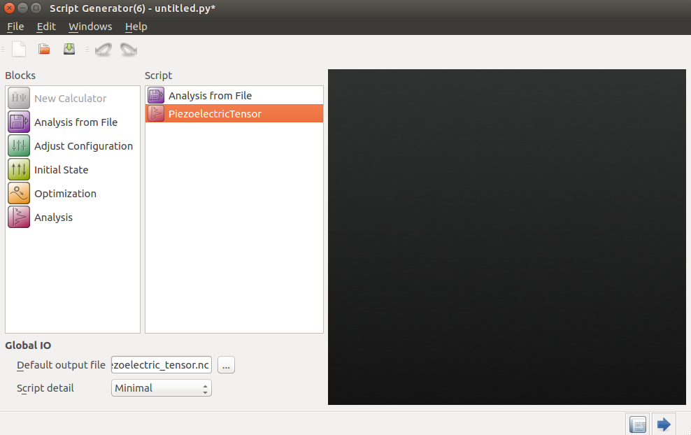
2. Double-click the Analysis from file block and select the object containing the optimized bulk structure (object id: gID001), as shown below.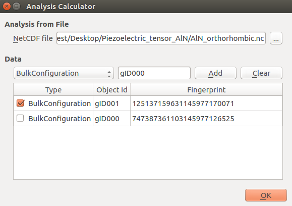

   

3. In the PiezoelectricTensor block, set the k-point sampling as in the next figure and tick “Optimize strained geometries”.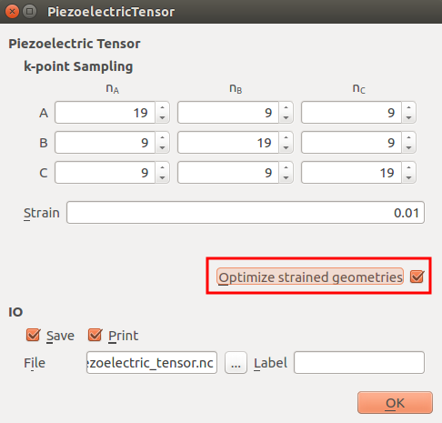

   

4. Save the HDF5 file and send the script to the Job Manager to run it.

Analysis of the \({e}_{33}\) coefficient

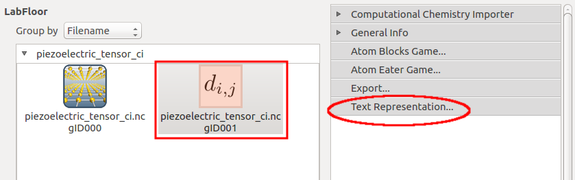
In the LabFloor, select the PiezoelectricTensor object and click the “Text Representation” plugin in the left hand panel to inspect the piezoelectric tensor.

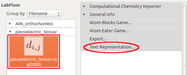
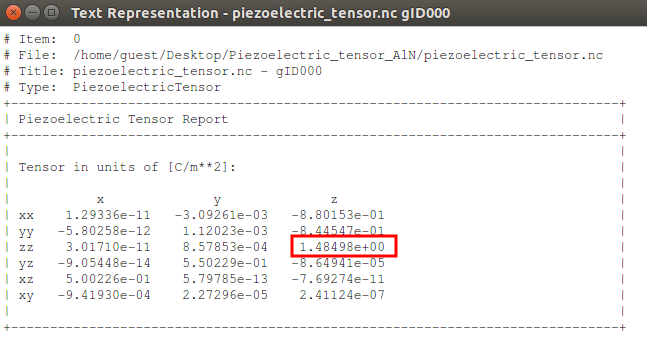
The predicted value for \({e}_{33}\) is 1.4849 C/m². This value is in good agreement with the value found in the literature (1.46 C/m²). [1]

In the next section we are going to see how you can calculate \({e}_{33}\) in an alternative way.

Alternative way of calculating the piezoelectric coefficient \({e}_{33}\)

The piezoelectric coefficient \({e}_{33}\) can be also calculated as the sum of two terms [1] [2]:

1. the clamped-ion term \({e}_{33}(0)\), that expresses the electronic response to strain.

2. a second term describing the effect of the internal strain on the piezoelectric polarization.

The complete expression for \({e}_{33}\) thus reads:

\[{e}_{33} = {e}_{33}(0) + \frac{4 e Z^{*}}{\sqrt{3} a^{2}} \frac{du}{d{\epsilon}_{3}}\]

where \(e\) is the electronic charge, \({\epsilon}_{3}\) is the macroscopic applied strain and \(Z^{*}\) is the Born effective charge, which depends on the change in polarization upon the dispacement of an ion (or rather, a periodic sublattice of equivalent ions):

\[Z_{\nu,i,j}^{*} = \frac{\Omega}{|e|} \frac{\partial {P}_{t}^{i}}{\partial{r}_{j}^{\nu}}\]

where \(\Omega\) is the unit cell volume, \({P}_t^i\) is the total polarization along the Cartesian direction \(i\), and \({r}^\nu_j\) is the coordinate of ion \(\nu\) in direction \(j\). The Born effective charge is also referred to as effective charge or dynamical charge.

Note

The Born effective charge is a tensor. Ìn fact, when an ion is displaced in direction \(j\), this will clearly affect the polarization in same direction \(j\). However, it may also lead to a change in polarization in another direction \(i\) perpendicular to \(j\).

In the calculations below the derivative will be approximated using finite differences:

\[\displaystyle \frac{\partial P_t^z}{\partial r^\nu_z} \approx \frac{P_t^z(+\delta \hat{z},\nu)-P_t^z(-\delta \hat{z},\nu)}{2\delta},\]

where \({P}_t^z(\pm\delta \hat{z},\nu)\) is the polarization along the z-direction when atom \(\nu\) has been displaced by the amount \(\delta\) in the positive/negative z-direction.

In the following, we will obtain \({e}_{33}\) by calculating each term explicitly. Specifically, we will:

1. calculate the variation of the interatomic distance due to strain \((\frac{du}{d{\epsilon}_{\alpha}})\);

2. compute the piezoelectric constant in the clamped-ion approximation \({e}_{33}(0)\);

3. compute the Born effective charge \({Z}^{*}\).

The variation of the interatomic distance due to strain

The AlN hexagonal cell

This variation is expressed as \(\frac{du}{d{\epsilon}_{\alpha}}\) where \({du}\) represents the difference in the interatomic distance \({u}\) (\({du}= {u'} - u\)) and \({d{\epsilon}_{3}}\) represents the applied strain (\({d{\epsilon}_{3}}= {c'} - c\)) in the direction parallel to the bond.

In order to calculate \({du}\) we will:

1. relax the bulk structure and calculate \({u}\);

2. apply a 1% strain to the unit cell in c direction, relax the internal parameters and get the interatomic distance under strain, \({u}^{'}\).

Calculating the interatomic distance \({u}\) for the relaxed system

1. Go to Builder and click Add ‣ Form Database, locate “AlN (Hexagonal)” in the database, and add it to the Stash.

   

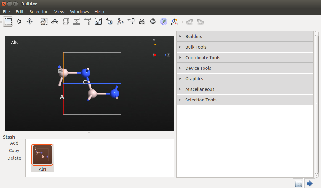
2. Send the bulk configuration to the Script Generator.

3. In the Script Generator, double-click the New Calculator and OptimizeGeometry (click Optimization ‣ Optimize Geometry) blocks to add them to the script.

   

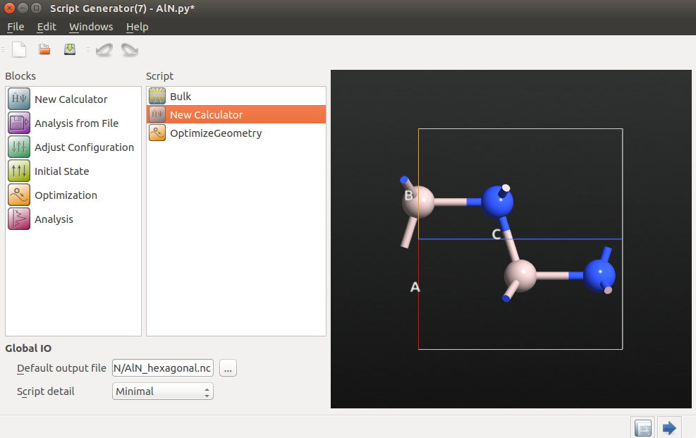
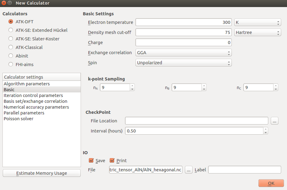
4. In the New Calculator block set the following parameters:

   • exchange and correlation: GGA.PBE

   • Basis set: DZP

   • k-point sampling: (9,9,9)

   

5. In the OptimizeGeometry block untick “Constrain Lattice Vectors”.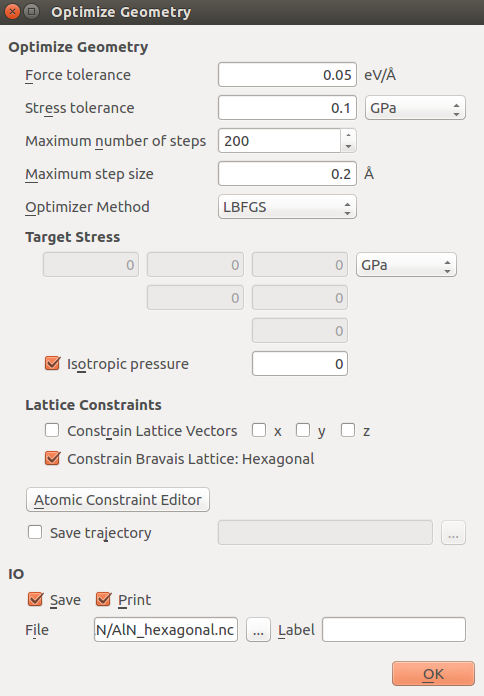

   

6. Save the HDF5 file as AlN_hexagonal.hdf5 and send the script to the Job Manager to run it.

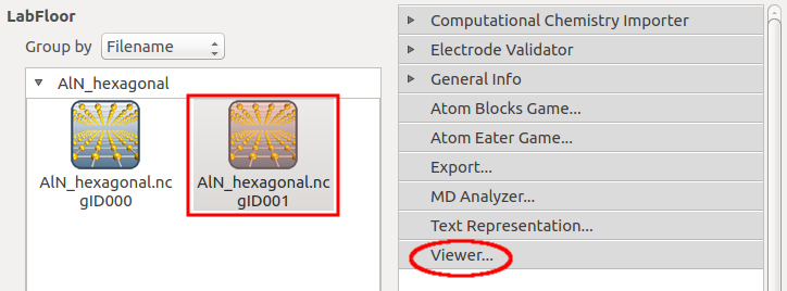
Once the job is finshed, the optimized bulk structure should appear in the LabFloor. Select it and click the Viewer plugin to visualize it.

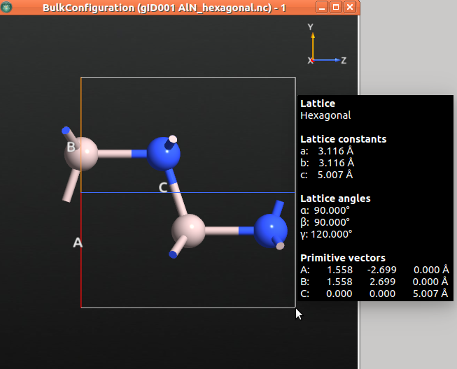
The table below shows the relaxed structural parameters.

Table 5 Table: Relaxed cell parameters in

	QuantumATK	Bernardini et al. [1]
a	3.116	3.0766
c	5.007	4.9810
c/a	1.607	1.6190
u/c	0.381	0.380

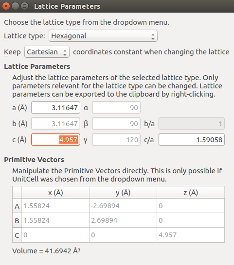
The value of the relaxed \({c}\) lattice constant is 5.007 Å. In the next step, we will apply a 1% compressive strain in the c direction by diminishing the lattice constant in c direction in 0.05 Å.

Internal relaxation under strain in z direction

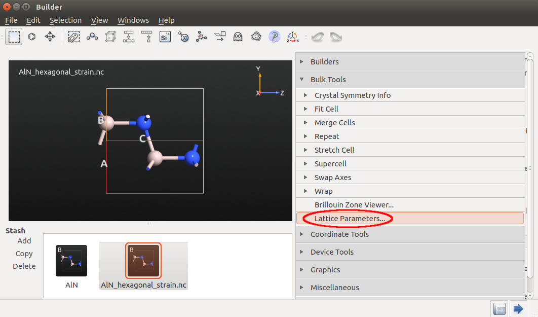
1. Send the relaxed structure to the Builder and rename it as AlN_hexagonal_strain.hdf5.

2. Go to Bulk Tools ‣ Lattice Parameters to decrease the lattice parameter in 1% in c direction.

   

   

3. Send the structure to the Script Generator to create a script.

4. In the Script Generator, double-click the New Calculator and OptimizeGeometry blocks.

5. In the New Calculator, set the following parameters:

   • exchange and correlation: GGA.PBE

   • k-point sampling: (9,9,9)

6. In the OptimizeGeometry block, constrain the lattice vectors as shown in the next figure.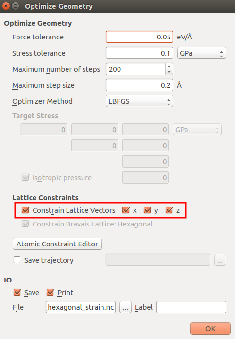

   

7. Send the script to the Job Manager and run the script.

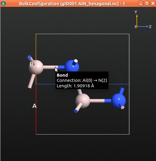
Once the calculation is finished, select the optimized bulk structure in the LabFloor and click the Viewer plugin to visualize the parameters.

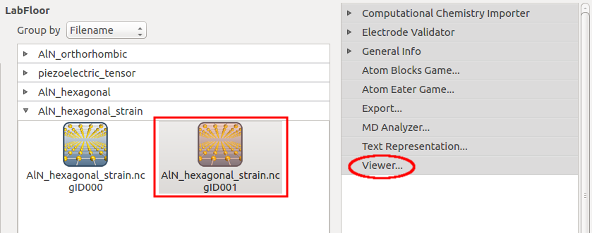
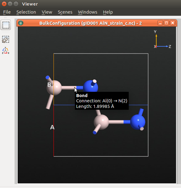
The predicted \({u'}\) value is 1.89985 Å, and therefore the predicted \(\frac{du}{d{\epsilon}_{3}}\) value is -0.1866. This value is in agreement with the value found in the literature (-0.18) [1].

Computing the piezoelectric tensor in the clamped-ion approximation

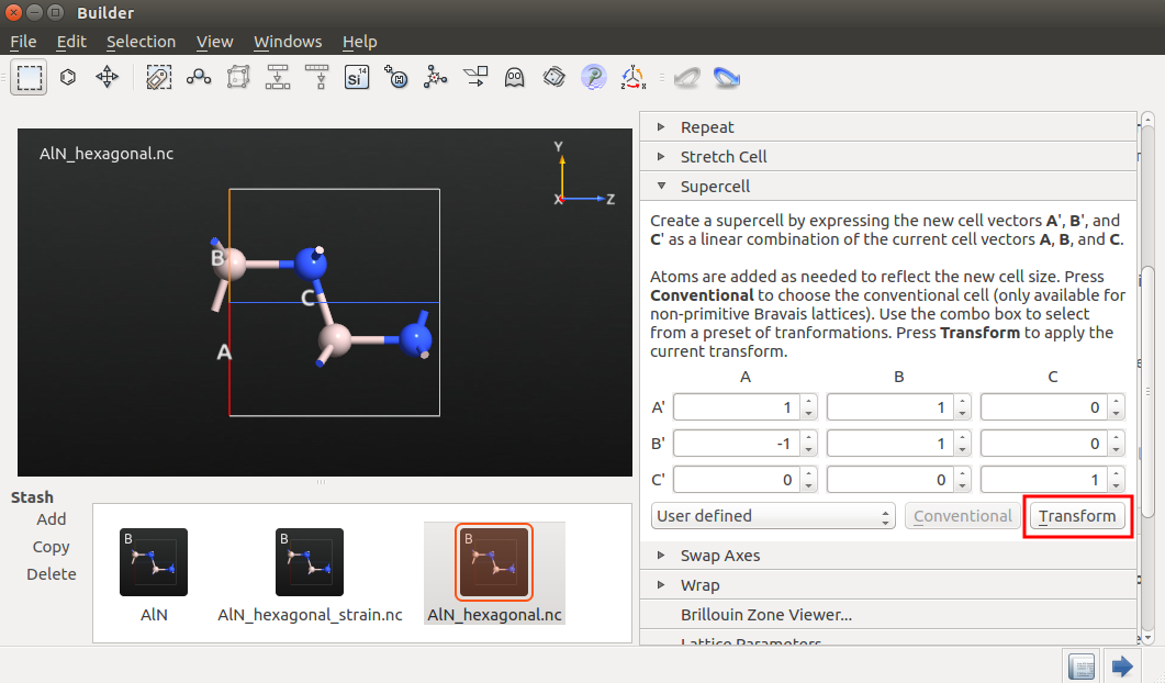
1. Send the relaxed structure to the Builder.

2. In the Builder, go to Bulk Tools ‣ Supercell to transform the cell according to the figure below.

   

3. Send the bulk configuration to the Script Generator and add the New Calculator and the Analysis ‣ PiezoelectricTensor blocks to the script.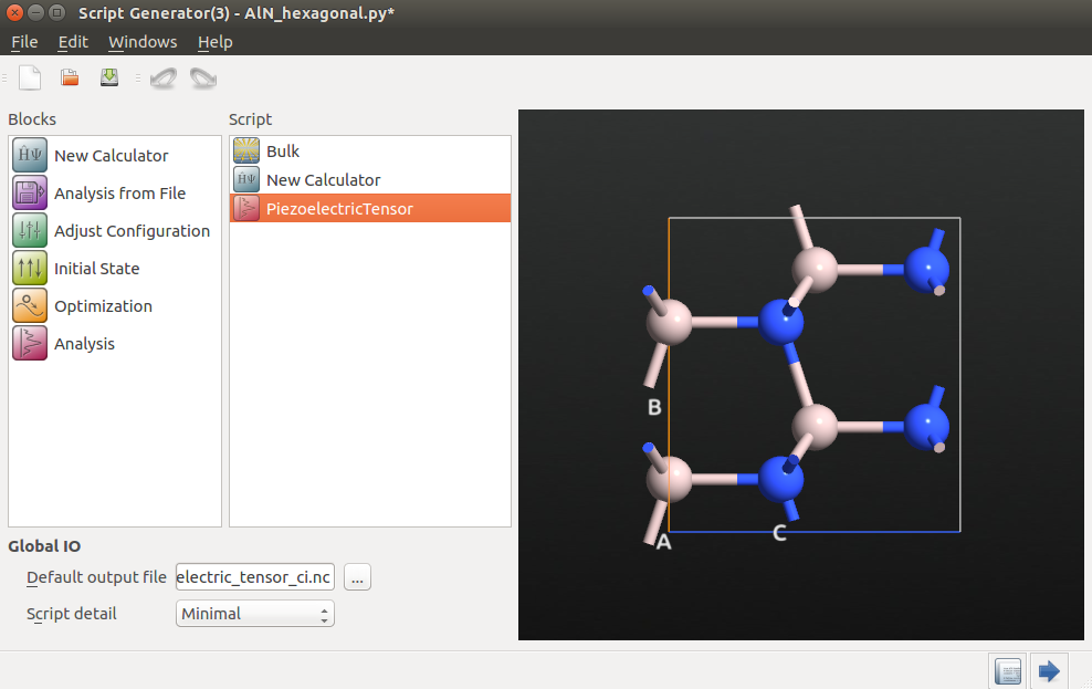

   

4. In the New Calculator block set the following parameters:

   • exchange and correlation: GGA.PBE

   • k-point sampling: (9,9,9)

5. In the PiezoelectricTensor block set a [(19,9,9), (9,19,9), (9,9,19)] k-point sampling as shown below.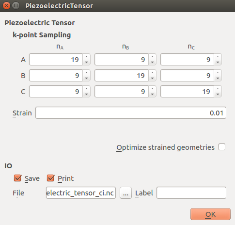

   

6. Save the HDF5 file as piezelectric_tensor_ci.hdf5 and send the script to the Job Manager to run it.

Once the calculation is finished, the PiezoelectricTensor object will appear in the LabFloor. Use the mouse to select the object and click the “Text Representation” plugin to visualize the tensor.

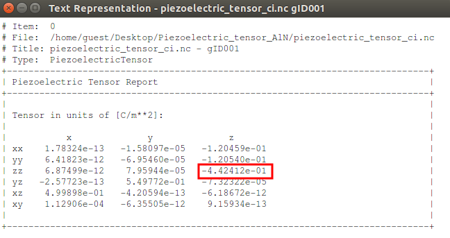
The predicted \({e}_{33}(0)\) value is -0.4424 C/m² , which is in good agreement with the value found in the literature [1].

Computing the Born effective charge

In order to compute the Born effective charge in QuantumATK, you need to use the script provided here (born_charges.py).

#read saved configuration
configuration0 = nlread('piezoelectric_tensor_ci.hdf5', object_id='gID000')[0]

# Get the fractional coordinates of read configuration
R0 = configuration0.fractionalCoordinates()

# Get the elements
elements = configuration0.elements()

# Get the lattice
lattice = configuration0.bravaisLattice()

# From the lattice extract unit cell volume and length of lattice vector in z-direction
volume = lattice.unitCellVolume()

vectors = lattice.primitiveVectors()
c = vectors[2][2]

# Get the calculator
calculator = configuration0.calculator()

# Number of atoms
numberOfAtoms = len(R0)

# Fractional displacement in the +/- z direction
delta_z = 0.01

# Array for storing the calculated Born Charges
bornCharges = numpy.zeros(numberOfAtoms)


# Loop over atoms in unit cell
for nAtom in range(numberOfAtoms):
    # Loop over displacement in positive/negative z-direction
    
    # List with polarization values
    Pz = []
    for s in [1,-1]:
        # Make a copy of the initial coordinates
        R = R0.copy()
        
        # Displace z-coordinate if atom 'nAtom'
        R[nAtom,2] += s*delta_z
        
        # Make a new configuration with the displaced atom
        configuration = BulkConfiguration(bravais_lattice=lattice,
                                                elements=elements,
                                                fractional_coordinates=R)
        
        # Set the calculator using the saved configuration as initial state
        configuration.setCalculator(calculator,initial_state=configuration0)
        
        # Update the configuration (DFT calculation)
        configuration.update()
        
        # Calculate polarization. Only use fine k-sampling in the z-direction
        polarization = Polarization(configuration=configuration,
                                    kpoints_a=MonkhorstPackGrid(2,2,2),
                                    kpoints_b=MonkhorstPackGrid(2,2,2),
                                    kpoints_c=MonkhorstPackGrid(5,5,20),
                                    )
        
        # Print polarization
        nlprint(polarization)
        
        # Get the total cartesian polarization
        Pt = polarization.totalCartesianPolarization()
        
        # Append the z-component to the Pz list
        Pz.append(Pt[2])
    
    # Make a finite difference approximation for the derivative
    dP = (Pz[0]-Pz[1])/(2*delta_z*c)
    
    # Calculate Born charge
    born_charge = volume*dP
    
    # Add the value (in units of electron charge) to the list 'bornCharges'
    bornCharges[nAtom] = born_charge.inUnitsOf(elementary_charge) 



# Finally print out the results
print('')
print('+------------------------------+')
print('| Born effective charges (e)   |')
print('+------------------------------+')

for nAtom in range(numberOfAtoms):
    print('  %2s' %elements[nAtom].symbol() + '  :      %4.4f       ' %bornCharges[nAtom]    )

print('+------------------------------+')
print('  Sum :      %4.4f       ' %numpy.sum(bornCharges))
print('+------------------------------+')

• The script starts reading the results from the previous calculation. This will serve as a good starting guess for the DFT calculations to be performed later in the script (where the atoms are displaced).

• Extract the fractional coordinates, the list of elements, the lattice, and the calculator from the configuration, and define a few convenient variables such as the unit cell volume and the length of the C lattice vector.

• The parameter delta_z is the fractional displacement when calculating the derivatives.

• There are two for loops in the script. The outer loop runs over the atoms in the unit cell, and the inner one (over the variable s) performs the displacements in the positive and negative z-direction.

• At the end of the script, the results are printed out.

Running the script

• Download the above born_charges.py script and save it in the Project Folder.

• Drag the script to the Job Manager to run it.

• When the job is finished, the calculated Born effective charges are written in the born_charges.log file.

• As indicated by the calculated sum of the Born effective charges, the calculated values fulfill the acoustic sum rule \(\sum_s Z_{s,ij}^*=0\) with only a small error.

You have already got all the components you needed to compute to calculate \({e}_{33}\). By substituting the computed values in the formula for \({e}_{33}\), you will obtain \({e}_{33} =\) 1.464 C/m², which is in good agreement with the value 1.4849 C/m² calculated above and with the value found in the literature (1.464 C/m²) [1].

References

[1] (1,2,3,4,5,6)

Fabio Bernardini, Vincenzo Fiorentini, and David Vanderbilt. Spontaneous polarization and piezoelectric constants of iii-v nitrides. Phys. Rev. B, 56:R10024–R10027, Oct 1997. doi:10.1103/PhysRevB.56.R10024.

[2]

T. Yokoyama, Y. Iwazaki, T. Nishihara, and M. Ueda. Analysis on electromechanical coupling coefficients in aln-based bulk acoustic wave resonators based on first-principle calculations. In Ultrasonics Symposium (IUS), 2012 IEEE International, 551–554. Oct 2012. doi:10.1109/ULTSYM.2012.0137.