Tuning the work function of silver by deposition of ultrathin oxide layers

Version: 2015.1

Downloads & Links

PDF version
MgO3LAg.py
MgO2LAg.py
MgO1LAg.py
Ag100.py
Basic QuantumATK Tutorial
ATK Reference Manual
Computing the work function of a metal surface using ghost atoms

Ultra-thin films of insulating materials deposited on a metal substrate constitute a peculiar class of materials with tunable properties and growing potential in different fields [1][2][3]. In this tutorial, you will learn how to change the work function of a substrate by depositing an overlayer of another material.

Note

Work function tuning
An important consequence of the deposition of a thin insulating film on a metal substrate is the induced change in work function of the metal support, which can be lowered or increased depending on the nature of the interface. Examples of such changes in work function have been reported in the literature. Kelvin probe force microscopy or scanning tunneling microscopy studies of alkali chloride thin films on Au(111) and Ag(100) have shown work function reductions of 0.5–1.2 eV [4][5]. Another work based on field-emission resonance has found for NaCl islands of up to 3 ML a work function reduction of 1.3 eV [6]. Theoretical calculations have predicted a reduction in work function for NaCl, MgO, and other oxides on various metals [7][8][9].

You will here calculate the work function change of a metallic Ag(100) surface as a consequence of depositing 1 to 3 layers of insulating MgO. The procedure to calculate the work function follows the prescription given in the tutorial Computing the work function of a metal surface using ghost atoms.

In particular, you will:

1. create and optimize the Ag and MgO bulk structures;

2. construct the Ag(100) and MgO(100) surfaces;

3. create the MgO(100)/Ag(100) interface;

4. set up work function calculations and run them;

5. analyze the results and compare with literature.

Warning

Computational settings
Throughout this tutorial you will use a particular set of computational settings (mesh cut-off, k-point sampling, basis-set, exchange-correlation, number of metal layers, etc.) which are chosen such that the QuantumATK results can be compared to literature. Always keep in mind, however, that you should check that your results are properly converged with respect to such settings.

Ag(100) and MgO(100) surfaces

Do the following to build the silver and magnesium oxide bulks:

• Open the Builder and click Add ‣ Add From Database, locate “Silver” in the database, and add it to the Stash.

• Also locate MgO and add it to the Stash. You should now have to bulk configurations in the Stash:

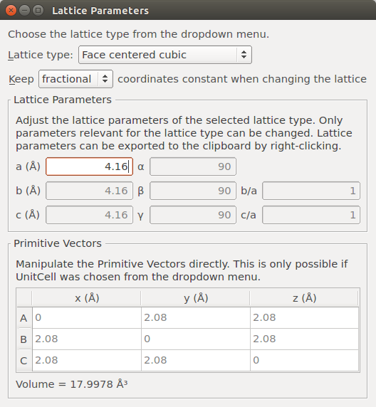
You will in this tutorial use the PW91 exchange-correlation functional for DFT simulations, in order to compare to literature results from Prada et al. [9]. The Ag lattice constant is 4.16 Å within PW91, so use this value for the silver bulk configuration:

• Select the “Silver” Stash item, and open the Bulk Tools ‣ Lattice Parameters plugin.

• Make sure fractional coordinates of the atoms are conserved when the lattice is changed, and enter 4.16 Å for the lattice parameter. Close the window.

Hint

You could also simply perform a DFT geometry optimization of the silver bulk configuration using PW91 and 11x11x11 k-points, and thereby relax the unit cell. The result of this more general approach would be approximately 4.16 Å for the lattice constant.

Next, create the Ag(100) surface:

• Use the Builders ‣ Surface (Cleave) tool to cleave the bulk silver along the [100] direction. Click Next twice.

• Choose Non-periodic and normal (slab) for the out-of-plane cell vector, and set the slab thickness to 5 layers with 15 Å top vacuum and 5 Å bottom vacuum. The large vacuum ensures that the effective potential can decay smoothly to zero above the slab.

Follow the same steps to create a 4-layer MgO(100) surface, and then rename the two new Stash items to “Ag(100)” and “MgO(100)”, respectively.

Ag/MgO interface

You should now use the Builders ‣ Interface plugin to create the Ag(100)/MgO (100) interface:

• Open the Interface plugin, and drag and drop the Ag(100) and MgO(100) configurations into the two drop zones. Notice that the Second surface (MgO) is automatically strained slightly, 0.81%, such that it matches the First surface (Ag):

• The Ag–MgO separation is way too large. Click the Shift Surfaces botton and enter a displacement along z of -19.4 Å in order to move the MgO(100) slab closer to the Ag(100). The interface separation should now be 2.7 Å. Note that an O atom is in an on-top position relative to an Ag atom, so you do not have to shift the MgO slab in the xy plane:

• Close the Shift Surfaces window and click Create to add the interface to the Stash.

Tip

You can learn more about the Interface Builder in the Technical Notes on Interface Builder.

DFT calculations

As explained in the tutorial Computing the work function of a metal surface using ghost atoms, you will need to add “ghost atoms” above the surface or interface. Work function calculations require a very good description of the charge density extending into the vacuum, and ghost atoms offer exactly this.

Adding ghost atoms

• Select the outermost O and Mg surface atoms (two atoms in total) and click the icon in the tool bar at the top of the Builder window:

• Next, swap the identity of the two ghost atoms, such that the O ghost atom is above the surface O atom and likewise for Mg. You can simply select a (ghost) atom and use the icon encircled in the image above to select from the periodic table.

• Finally, send the configuration to the Script Generator .

ATK-DFT calculations

The work function is identified as the chemical potential when the effective potential is zero on the cell boundary above the surface. A Dirichlet boundary condition (BC) is used to enforce this. You will also compute the effective potential in order to inspect it visually. Set up the required DFT calculations in the following manner:

• Change the default output name to MgO3LAg.nc and add four blocks to the script: New Calculator, OptimizeGeometry, ChemicalPotential, and EffectivePotential.

• Open the New Calculator block and set the following parameters:

  • k-point Sampling: 11x11x1;

  • Iteration Control: Tolerance = 10^-5 Hartree;

  • Exchange Correlation: GGA.PW91;

  • Basis set: DoubleZetaPolarized for O and Mg, SingleZetaPolarized for Ag;

  • Poisson solver:

    • choose the FFT2D solver,

    • select a Neumann BC on the left C face,

    • select a Dirichlet BC on the right C face.

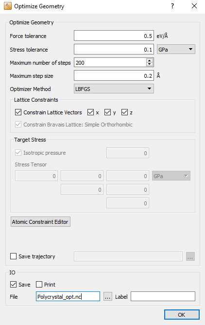
• Next, open the OptimizeGeometry block and edit it. In particular, make sure to constrain the bottom of the Ag(100) slab and the ghost atoms during the optimization:

  • Decrease the force tolerance to 0.01 eV/Å.

  • Tick Save trajectory, and enter MgO3LAg.nc as the file name.

  • Click Add Constraints and select the bottom two Ag atoms and the two ghost atoms. Then click Add tag from selection and choose a Fixed constraint for that group (Selection 0).

• Save the script as MgO3LAg.py and execute it using the Job Manager . If needed, you can also download the final script here: MgO3LAg.py. It should only take about five minutes to finish if executed in serial on a modern laptop. This can be reduced to 2.5 minutes if executed in parallel with 4 MPI processes.

Analyzing the results

The OptimizeGeometry, ChemicalPotential and EffectivePotential objects should now have appeared on the QuantumATK LabFloor:

OptimizeGeometry
ChemicalPotential
EffectivePotential

Try to select the OptimizeGeometry object and visualize the relaxation trajectory by clicking the Viewer plugin on the right-hand side of the LabFloor. Click to start the video. Confirm that the constrained Ag and ghost atoms are indeed fixed during relaxation.

Work function

Select the ChemicalPotential object and click the Show Text Representation plugin to read off the calculated chemical potential of -2.99 eV.

The work function for this 3 layer MgO on Ag(100) is therefore 2.99 eV, which is in a very good agreement with the calculated value of 2.96 eV reported in the literature by Prada et al. [9].

You can also create the 2L-MgO/Ag(100), 1L-MgO/Ag(100) and the Ag(100) systems following the steps described above. Another approach is to use the relaxed 3L-MgO/Ag(100) configuration as a starting point for the other systems. This will reduce the number of BFGS steps needed for relaxing those systems, and thereby save computational time.

For example, to create the 2L-MgO/Ag system and calculate the work function:

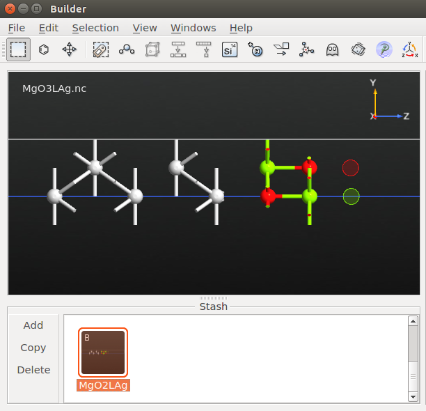
• Locate the relaxed 3L-MgO/Ag(100) configuration on the LabFloor. It has object ID glD002.

• Transfer it to the Builder and rename it MgO2LAg.

• Delete the two O and Mg ghost atoms, and convert the new surface O and Mg atoms to ghost atoms.

• Swap the Mg and O ghost atoms as described above.

• Send the configuration to the Scripter and set up the calculation as descibed above.

Table 4 Table: Calculated PW91 work functions (eV). The corresponding work function difference wrt. to clean Ag(100) is reported in parenthesis.

	QuantumATK	Pada et al. [9]
Ag(100)	4.22	4.23
1L-MgO/Ag	3.31 (-0.91)	3.29 (-0.94)
2L-MgO/Ag	2.97 (-1.25)	2.95 (-1.28)
3L-MgO/Ag	2.99 (-1.23)	2.96 (-1.27)

The scripts needed to calculate all the work functions in the table column labelled QuantumATK may be downloaded here: Ag100.py, MgO1LAg.py, MgO2LAg.py, MgO3LAg.py.

Tip

The table above shows excellent agreement between QuantumATK and literature (VASP) work function calculations. However, results may change if the computational settings change. For example, a SZP basis set was used for the Ag atoms – a DZP basis set may give slightly different results. The type of pseudopotentials used may also affect results, and more ghost atoms may be needed in some cases.

Effective potential

You have used a particular set of boundary conditions for the work function calculations – Neumann on the left C face, and Dirichlet on the right C face. You can now use the 1D Projector plugin to visualize the average effective potential in the calculations:

• Select the EffectivePotential object on the LabFloor, and click the 1D Projector plugin.

• Select to project along the C axis using the Average projection type, and click Add line to plot the projection:

The effective potential is clearly different in the Ag(100) and MgO(100) regions. Moreover, the effect of the two different BCs are quite clear from the value and slope of the potential in both ends of the supercell:

• The Neumann BC on the left C face has imposed a zero slope of the effective potential on the boundary, but does not constrain the actual value of the potential on the boundary.

• On the contrary, the Dirichlet BC on the right C face has forced the effective potential to zero on the boundary, and the slope just happens to be approximately zero in the vacuum region.

1D Projector plugin

Common QuantumATK grid objects

BlochState, EffectivePotential, Eigenstate, ElectronDensity, ElectronDifferenceDensity, ElectrostaticDifferencePotential, ExchangeCorrelationPotential, ExternalPotential, LocalDeviceDensityOfStates, TransmissionEigenstate, ElectronLocalizationFunction.

The 1D Projector can be used to project all sorts of 3D grid data onto a 1D representation. This is very useful for visualization purposes, and works for a wise range of QuantumATK grid objects (see the box).

Several options are available in the plugin widget:

Grid

You can open the projector tool with multiple objects selected on the LabFloor, to plot them next to each other. Here you choose which one to plot.

Axis

Choose along which direction you want to project your 3D data grid.

Projection type

Sum or average all the data in the plane perpendicular to the selected direction. You can also simply plot the single values along a line passing through a particular projection point.

Projection point

Specify, in fractional coordinates, the projection point to be used in case the projection type Through point is selected.

Spin projection

In case of spin polarized calculations, collinear or non-collinear, you can select the specific spin projection.

Add line

Once the options above are specified, click this button to plot your projection in the window on the right-hand side. You can add more projections to the same plot.

Remove line

Select one line in the Projection Plot window and click to remove the line from the plot.

Clear plot

Remove all lines from the plot.

Line Info

Some useful information about the currently selected plot line/point are shown. Note that the plot is interactive. Click on any point of the plot to print the corresponding information.

Projection Plot

Right-click to zoom, customize or export data to file.

References

[1]

Livia Giordano and Gianfranco Pacchioni. Oxide films at the nanoscale: new structures, new functions, and new materials. Accounts of Chemical Research, 44(11):1244–1252, 2011. doi:10.1021/ar200139y.

[2]

Gianfranco Pacchioni. Two-dimensional oxides: multifunctional materials for advanced technologies. Chemistry – A European Journal, 18(33):10144–10158, 2012. doi:10.1002/chem.201201117.

[3]

Gianfranco Pacchioni and Freund Hajo. Electron transfer at oxide surfaces. the mgo paradigm: from defects to ultrathin films. Chemical Reviews, 113(6):4035–4072, 2013. doi:10.1021/cr3002017.

[4]

Christian Loppacher, Ulrich Zerweck, and M. Lukas Eng. Kelvin probe force microscopy of alkali chloride thin films on au(111). Nanotechnology, 15(2):S9, 2004. URL: http://iopscience.iop.org/article/10.1088/0957-4484/15/2/003/meta.

[5]

Marina Pivetta, Fran\ifmmode \mbox ç\else  ç\fi ois Patthey, Massimiliano Stengel, Alfonso Baldereschi, and Wolf-Dieter Schneider. Local work function moiré pattern on ultrathin ionic films: nacl on ag(100). Phys. Rev. B, 72:115404, Sep 2005. doi:10.1103/PhysRevB.72.115404.

[6]

Hans-Christoph Ploigt, Christophe Brun, Marina Pivetta, Fran\ifmmode \mbox ç\else  ç\fi ois Patthey, and Wolf-Dieter Schneider. Local work function changes determined by field emission resonances: nacl∕ag(100). Phys. Rev. B, 76:195404, Nov 2007. doi:10.1103/PhysRevB.76.195404.

[7]

G. Butti, M. I. Trioni, and H. Ishida. Electronic properties calculation of mgo thin films adsorbed on semi-infinite ag(001). Phys. Rev. B, 70:195425, Nov 2004. doi:10.1103/PhysRevB.70.195425.

[8]

Livia Giordano, Fabrizio Cinquini, and Gianfranco Pacchioni. Tuning the surface metal work function by deposition of ultrathin oxide films: density functional calculations. Phys. Rev. B, 73:045414, Jan 2006. doi:10.1103/PhysRevB.73.045414.

[9] (1,2,3,4)

Stefano Prada, Umberto Martinez, and Gianfranco Pacchioni. Work function changes induced by deposition of ultrathin dielectric films on metals: a theoretical analysis. Phys. Rev. B, 78:235423, Dec 2008. doi:10.1103/PhysRevB.78.235423.