Organize your data in the Nanolab data view

Working with ab-initio simulations require a lot of data and it can be challenging to manage and organize data from many different simulations.

When opening Nanolab. the first window that shows up, is the Nanolab data view. The Nanolab data view makes it possible to filter, analyze and summarize all the constructed structures and calculated results.

The Nanolab Data View

This introduction to the Nanolab data view, will explain the 6 main parts of the data view:

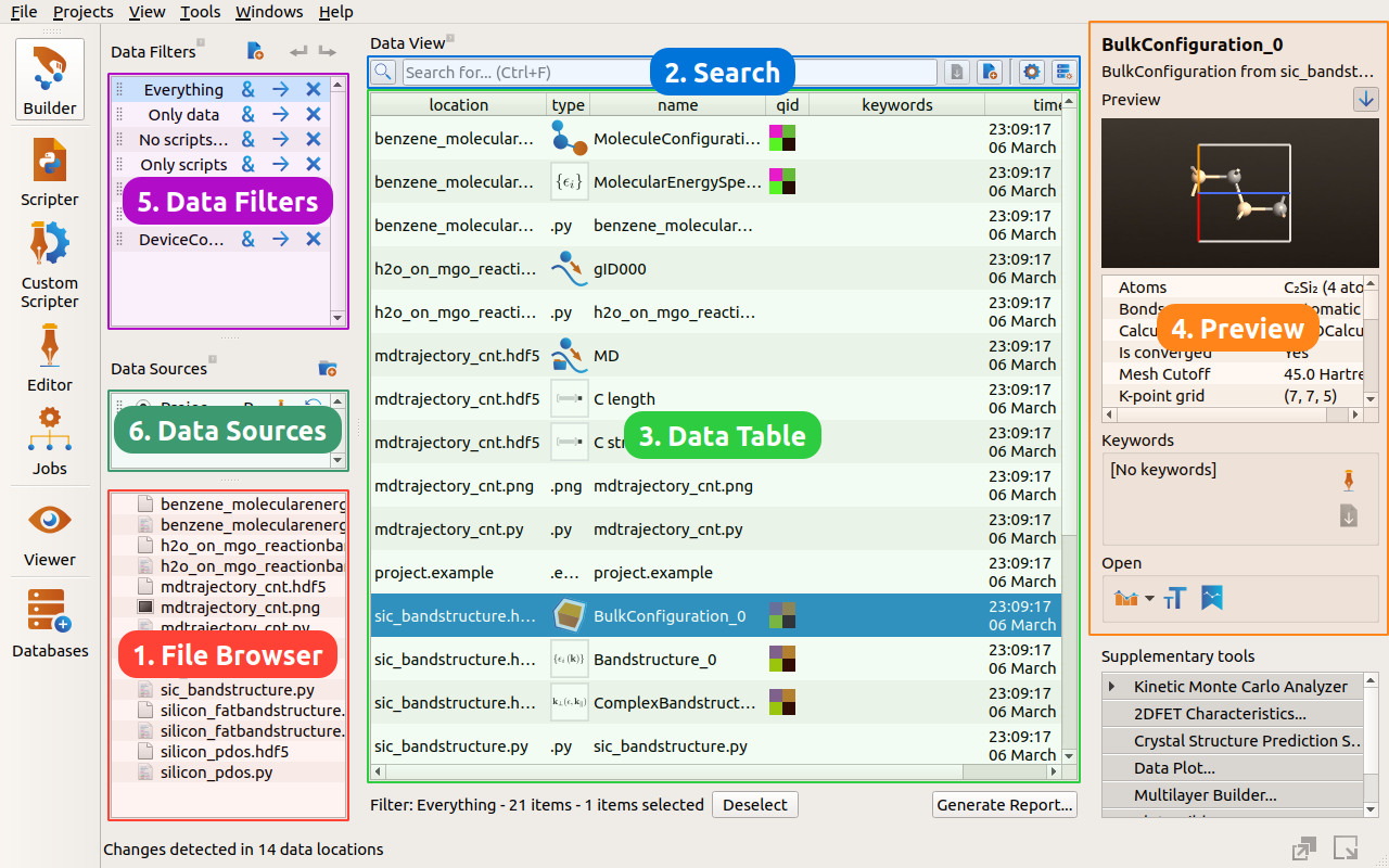
1. The File Browser

The tutorial starts in the lower left corner, where you will find a familiar file browser showing the contents of the current project folder.

Select a file, and the data table (to the right of the file browser) will display the structures and results saved in that file. Select multiple files by holding down ctrl or shift while clicking the files with the mouse.

2. The Search Field

It is also possible to search through your data using the search bar at the top of the Nanolab data view. Type in search queries to quickly locate your data. Note that it will search across several columns in the data view – including folders, filenames, data type, object ids and keywords.

This makes it possible to quickly find, e.g. all Bandstructures or MDTrajectories within a relevant folder.

It is also possible to use more advanced SQL queries to create custom views on your data. It make take some effort to create the most powerful queries, and therefore the queries can be saved as what we call “Data filters”. Such saved filters can quickly be applied and combined with other queries in order to properly limit your search.

The advanced SQL search

In addition to normal free-text search terms, the search field also accepts SQL queries. It is even possible to combine text search and SQL search together in the search field. Here are some examples of how the search field can help locate relevant data.

This query search for all results of type ‘Bandstructure’:

type='Bandstructure'

This query searches for all data items that have a name starting with “Electron”. Note the use of the % sign to signify wild card matching.

name LIKE 'Electron%'

In addition to searching, the data can be sorted by e.g. the last changed time. Here the specifier ASC sorts the timestamp in ascending order. Similarly sorting can be done in descending order by using the DESC specifier.

name LIKE 'Electron%' ORDER BY timestamp ASC

Multiple queries can be joined by “OR” or “AND”. Here we search a specific subfolder for all bandstructures.

location LIKE 'my_subfolder%' AND type="Bandstructure" ORDER BY timestamp ASC

Also, normal search terms can be combined with SQL. Let us search for anything related to ‘silicon’ of type ‘Bandstructure’ and ordered by timestamp.

type='Bandstructure' AND silicon ORDER BY timestamp ASC

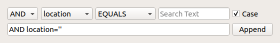
The Query Builder

Advanced SQL-searches can be difficult to master, and as a help Nanolab provides the advanced query builder. Click the cog-button to show the query builder. Fill in menus and text fields to construct the relevant queries.

3. The Data Table

The main data table shows all the data that matches the current search query. Each piece of data is represented as a single row in the table (in the following called a data item).

The columns displays the data location (folder and filename), data type, object id, Quantum ID (qid), keywords and last changed time.

Each data item can be double clicked. This will open a window with a relevant analysis, that will display the scientific data contained in the data item. Try double-clicking an atomic structure to open the 3D Viewer, a Bandstructure to show a plot of the band diagram or an MDTrajectory to show the time-evolution.

For more detailed options, right-click a data item. This will open a detailed menu with several options:

• Open. This will open the default analysis.

• Open with. Displays a menu of all available analysis for this data type.

• Delete. Some items support deletion. Note that deletions cannot be undone.

• Unpack. Show nested data (see explanation below).

• Export the selected data items to specific file formates (.hdf5, .xyz, .mol and so forth).

• Refine the search field based on the right-clicked data item, by choosing “Refine …”

The Quantum ID (qid)

Calculations done with LCAOCalculator, PlaneWaveCalculator or SemiEmpericalCalculator are all marked with a unique number called a quantum ID (qid). The number can be cumbersome to work with, so in the data view it has been encoded as 4 colors. The four-colored squares can quickly be used to distinguish different calculations, since analysis done with the same calculator all share the same quantum ID.

Unpack

Some data may contain nested data. MDTrajectories will for example sometimes contain custom measurements of stresses and strain. All data items containing nested data are marked with a folder-like unpack icon .

Right click one of these items and choose “Unpack” to show the contents of the data. The nested data can then be inspected and analyzed like all other data.

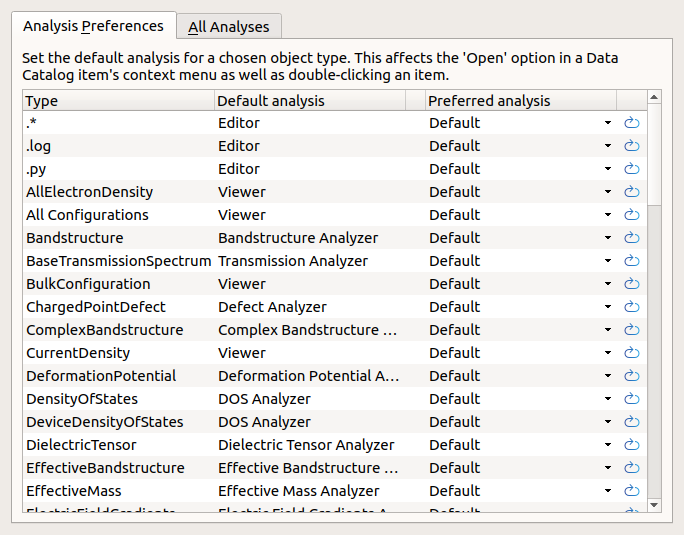
Analyzers and Preferences

Double-click a data item to open it with it’s default analyzer. Bandstructures will open to reveal the band diagram, atomic structures will open in the 3D Viewer and so forth. Additional analyzers can always be found in the right-click menu.

It is possible to change the default analysis for a given type of data. Open the analysis preferences by clicking the bookmark button and you are presented with a list of types and analyzers. For each analyzer you can see the default and make a user-defined change. Those changes apply across all projects.

4. The Data Preview

Clicking a data item will display a preview of the relevant data in the preview panel to the right of the data table.

For atomic structure configurations the preview includes a 3D view of the atomic structure along with relevant data like bonds and unique elements. If the structure has a calculator attached, it is also possible to inspect the calculator settings. Many different data types items expose some results or settings in the preview pane.

The 3D view can be disabled by clicking the arrow-down button. This may be convenient when working on slower machines or with very large structures.

The Keywords

Data items can also be annotated by keywords that can be used for categorization and search. Atomic structures will also automatically embed the unique elements and its calculator name as keywords.

The preview panel also contains a keyword editor, where it is possible to add custom keywords to your data items. This can be a convenient way to attach additional data to your data items, or for enabled special searches or filters.

5. The Data Filters

In the upper left corner is a list of saved searches known as Data Filters. Per default each project starts with a few standard filters that has been given appropriate names. The Only molecules filter for example corresponds to the advanced search query type='MoleculeConfiguration'.

Each filters can be applied by clicking their arrow button . This will replace the currently active search query with the filter query. It is also possible to combine multiple filters by using the button.

This “&” feature makes it very easy to perform advanced searches like for example “all molecules within the MyStructures folder”:

1. Click the MyStructures folder in the folder view.

2. Click the next to the “Only molecules” default filter.

6. The Data Sources

The data sources specify what data belong in the current project. The table shows the list of current sources.

Each project always a contains single folder (the project folder) as the main data source, but it is possible to add additional folders as sources. Simply click the button and navigate to the desired folder in order to add it to the current project.

Each source has a unique name. The project folder is always named P while subsequent sources are named S0, S1, etc. Clicking the source name will limit the search to the corresponding source by changing the search query to e.g.,

source='S0'

The settings for each data source can be accessed by clicking the pen button . In these settings the current source folder can be changed along with the activated data inspectors.

Data Inspectors

A data inspector can turn files into data in the data table. A standard source is capable of automatically import data from QuantumATK files, .xyz files, .cif files, LAMMPS files, VASP files and QuantumEspresso files.

However, NanoLab supports many different file format inspectors that can be activated in the settings menu. Simply tick off the desired inspectors to enable them, and wait a few seconds for Nanolab to re-index the files.