Graphene nanoribbon device: Electric properties

The purpose of this tutorial is to show you how the ATK-SE package can be used to calculate the electric properties of a nano-scale transistor device. You will compute quantities like the electron transmission spectrum, conductance, I–V curve, and electron thermal transport.

Attention

Graphene nanoribbon device with a gate and a dielectric spacer

The device system considered in this tutorial consists of a z-shaped graphene nanoribbon on top of a dielectric and controlled by a metallic gate, as illustrated below. It forms a metal–semiconductor–metal junction. By applying a gate potential across the central region, the system can function as a field effect transistor (FET).

Attention

This tutorial assumes that you have already built the small nanoribbon transistor as described here: Small nanoribbon transistor. If you have not, please do so before continuing with this tutorial.

Fig. 87 The device system considered in this tutorial consists of a z-shaped graphene nano-ribbon, on top of a dielectric and controlled by a metallic gate. The contour plot illustrates the electrostatic potential through the system.

The device is illustrated in the figure above. It consists of three regions; a central region and two electrodes. You will calculate the following properties of the system.

• Transmission spectrum

• Temperature dependent conductance

• Temperature induced current

• Conductance as function of gate potential and temperature

• Current as function of bias, gate potential and temperature

Get started

Create a new QuantumATK project and add the already built nanoribbon device to the project:

• Open the Builder and use Add ‣ From Files to find the saved device_configuration (in QuantumATK Python or HDF5 format) and add it to the Stash.

Electron transmission spectrum

Send the configuration from the Builder to the Scripter by using the icon in the lower right-hand corner of the Builder window.

Then set up the semi-empirical electron transmission calculation. Add the following blocks to the script:

• New Calculator

• Analysis ‣ ElectronDifferenceDensity

• Analysis ‣ ElectrostaticDifferencePotential

• Analysis ‣ TransmissionSpectrum

Then change the output filename to z-a-z-6-6.hdf5.

Calculator settings

Open the calculator block and edit the settings:

• Select the ATK-SE: Extended Hückel (Device) calculator, and lower the number of k-points in the C direction to 50, which should be sufficient for this calculation.

• Uncheck the No SCF iteration box, to perform a self consistent calculation.

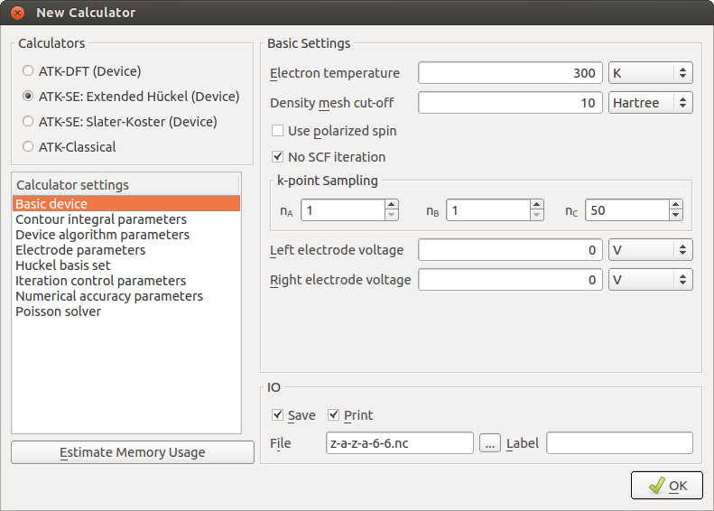
• The next step is to change the basis set for the calculation to use parameters specifically optimized for describing carbon structures [1]. To this end, enter the Huckel basis set menu and select the Cerda.Carbon [Graphite] and Hoffmann.Hydrogen basis sets.

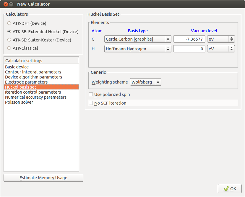
Note

The default vacuum level for each basis set is chosen such that the carbon and hydrogen parameters they can be used together, even though they are fitted to different reference systems.

• Make sure to use the “Multigrid” Poisson solver and “Neumann” boundary conditions along the A and B directions, which are perpendicular to the transport direction. See the image below.

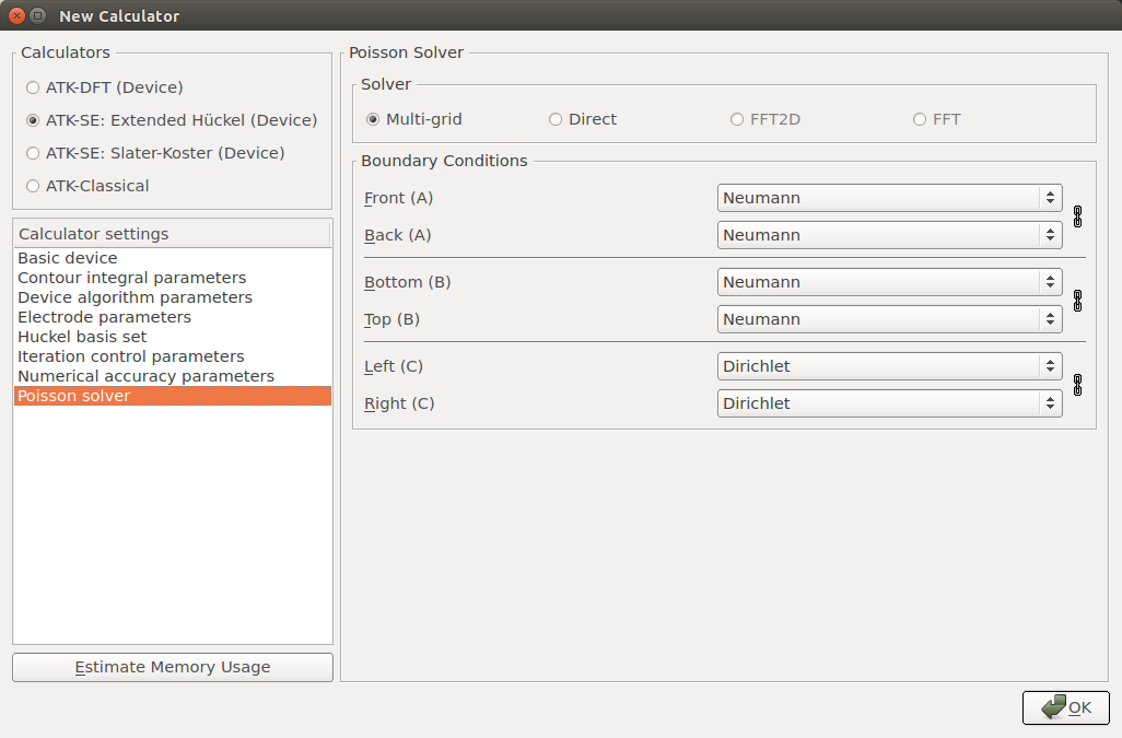
Attention

It is import to use Neumann boundary conditions along non-periodic directions perpendicular to C, when your device has a metallic gate. Why is this?

The Neumann boundary condition imposes the constraint that the derivative of the electrostatic potential should be zero on that boundary. Put diffferently; the electrostatic potential should be constant at the boundary (but make take on any value). This is the appropriate boundary condition when the device has a metallic gate!

Setup the analysis blocks

• Keep the default settings in the ElectronDifferenceDensity and ElectroStaticDifferencePotential blocks.

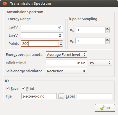
• In TransmissionSpectrum, increase the number of sampling points to 200.

You have now completed setting up the calculation. Save the script in the project directory as z-a-z-6-6.py.

Run the calculation

Execute the calculation by sending the script to the Job Manager, again using the botton. You may be asked to save the script again. Click the botton to start the job. It will take 5 to 15 minutes, depending on your computer.

Note

What is actually happening during the calculation?

The job will first perform a self-consistent calculation for each of the electrodes. The self-consistent electrode Hartree potential is then used as a boundary condition in a self-consistent calculation for the central region of the device. Finally, the transmission spectrum and other analysis objects of the structure are calculated.

Tip

If you accidentally closed down the Scripter window, or even the QuantumATK main window, your work is not lost! You can simply drag-and-drop the saved Python scipt onto the Scripter to open it for editing. Similarly, you can directly send any saved script to the Job Manager.

Examine the results

Transmission Spectrum

Switch to the QuantumATK main window, where you will note that the HDF5 file z-a-z-6-6.hdf5 has been generated. The contents of the file should already be displayed on the LabFloor. It contains the DeviceConfiguration and the requested analysis objects:

• ElectronDifferenceDensity

• ElectrostaticDifferencePotential

• TransmissionSpectrum

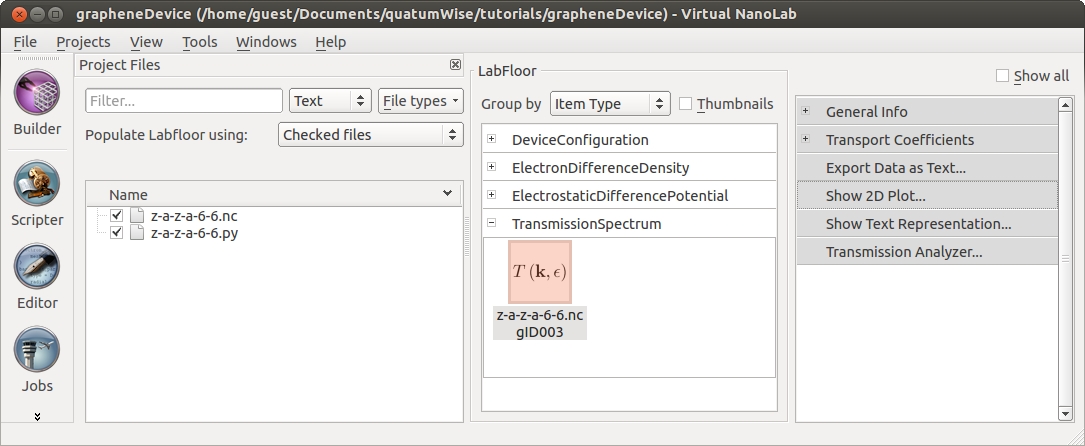
Select the TransmissionSpectrum object and use the 2D Plot plugin to visualize the calculated transmission spectrum.

Note

The transmission spectrum has a low value in the energy range [-0.5, 1.5] eV, corresponding to the energy window within the band gap of the central semi-conducting armchair-edge ribbon. The asymmetric position of the electrode Fermi levels relative to the band edges, i.e. the shift of the valence band edge of the central region towards the electrode Fermi levels, is due to the applied gate potential of -1V.

Electrostatic potential

To visualize the effect of the gate potential, select the ElectrostaticDifferencePotential object and click the Viewer plugin. Select Contour Plot from the dialogue that pops up.

To make the plot more interesting, add a 3D rendering of the graphene junction by dropping the DeviceConfiguration from the LabFloor onto the open scene in the Viewer. Then rotate the contour plot:

• Click Properties and select CutPlanes from the top.

• Change the rotation angle, \(\theta_y\), to 151° and set the color map to RGB.

• Finally, rotate the camera of the 3D view with the mouse to obtain a plot similar to the image shown below.

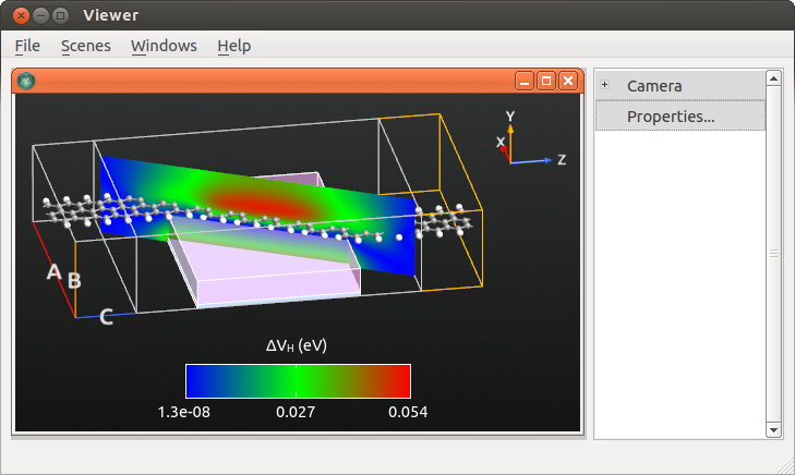
If you wish to export a copy of the contour plot, right-click in the Viewer window, and choose Export (or use Ctrl+E). You can choose to export as PNG og JPG graphics. The image is now stored on disk and can be used for further processing in any other third party application of your choice.

Effect of the Gate Potential

You will now investigate the effect of changing the gate potential. In the previous section, the gate potential was fixed at -1 V. You will now vary the potential in the range of [-2,2] V and calculate the transmission spectrum at each gate potential.

Gate potential loop

For each value of the gate potential you should perform a new self-consistent calculation to obtain the corresponding transmission spectrum. Such a loop is conveniently done by the following QuantumATK script. You can download it here: gate_loop.py

#read in the old configuration
device_configuration = nlread("z-a-z-6-6.nc",DeviceConfiguration)[0]
calculator = device_configuration.calculator()
metallic_region0 = device_configuration.metallicRegions()[0]
# Define gate_voltages
gate_voltage_list=numpy.linspace(-2.0,2.0,17)*Volt
for gate_voltage in gate_voltage_list:
    # set the gate potential
    device_configuration.setMetallicRegions(
        [metallic_region0(value = gate_voltage)] )
    # make a copy of the calculator and attach it to the configuration
    # restart from the previous scf state
    device_configuration.setCalculator(calculator(),
        initial_state=device_configuration)
    #Analysis
    filename= 'gatescan-6-6.nc'
    electron_density = ElectronDifferenceDensity(device_configuration)
    nlsave(filename, electron_density,object_id='dens'+str(gate_voltage))
    electrostatic_potential = ElectrostaticDifferencePotential(device_configuration)
    nlsave(filename, electrostatic_potential, object_id='pot'+str(gate_voltage))
    transmission_spectrum = TransmissionSpectrum(
        configuration=device_configuration,
        energies=numpy.linspace(-2,2,200)*eV,
        )
    nlsave(filename, transmission_spectrum,object_id='trans'+str(gate_voltage))
    nlprint(transmission_spectrum)

The script implements the following workflow:

1. Read the self-consistent calculation obtained in the previous chapter and use this as the starting point for the calculations:

#read in the old configuration
device_configuration = nlread("z-a-z-6-6.nc",DeviceConfiguration)[0]
calculator = device_configuration.calculator()
metallic_region0 = device_configuration.metallicRegions()[0]

2. Set up a list of gate voltage values [-2.0, -1.75, …, 2.0]*Volt:

   # Define gate_voltages
   gate_voltage_list=numpy.linspace(-2.0,2.0,17)*Volt
   

3. Loop through the gate voltage list, and for each value modify the value of the gate voltage in the metallic region:

for gate_voltage in gate_voltage_list:
    # set the gate potential
    device_configuration.setMetallicRegions(
        [metallic_region0(value = gate_voltage)] )

4. Initialize the self-consistent state of the device configuration by calling the calculator() method.

       # make a copy of the calculator and attach it to the configuration
       # restart from the previous scf state
       device_configuration.setCalculator(calculator(),
           initial_state=device_configuration)
   

   This method will make a copy of the previous Huckel calculator using the same settings. Since a new calculator is attached, a self-consistent calculation will automatically be performed the next time a property of the system is required:

5. Finally, the same analysis objects as in the previous chapter are calculated and save them into a HDF5 file. Note that for each analysis object a specific object_id is specified. This will make it easier to retrieve the correct entries from the HDF5 file:

       #Analysis
       filename= 'gatescan-6-6.nc'
       electron_density = ElectronDifferenceDensity(device_configuration)
       nlsave(filename, electron_density,object_id='dens'+str(gate_voltage))
       electrostatic_potential = ElectrostaticDifferencePotential(device_configuration)
       nlsave(filename, electrostatic_potential, object_id='pot'+str(gate_voltage))
       transmission_spectrum = TransmissionSpectrum(
           configuration=device_configuration,
           energies=numpy.linspace(-2,2,200)*eV,
           )
       nlsave(filename, transmission_spectrum,object_id='trans'+str(gate_voltage))
       nlprint(transmission_spectrum)
   

Run the script using the Job Manager or execute it from a terminal:

$ atkpython gatescan-6-6.py > gatescan-6-6.out

The script will take a while to complete, since 17 self-consistent calculations are needed. The total execution time may be between 2 and 8 hours, depending on your hardware.

Conductance as a function of gate potential

The script in the previous section produced the data file gatescan-6-6.hdf5. It should contain all the calculated transmission spectra. Try to inspect them using the Transmission Analyzer to see how the transmission spectrum changes with the gate potential.

Note

You will find that all the spectra look rather similar and that the main difference between the different spectra is a shift of the valence and conduction band edges relative to the Fermi level.

This is the main function of the metallic gate: It can be used to tune the band edge positions relative to the Fermi level, and thereby control the electric properties of the device!

You will now use the data to calculate the conductance of the junction as a function of the gate potential for different electrode temperatures. Use the following script, which is a slight modification of the script used in the previous chapter. You can also download it here: conductance_diff_gate.py.

#make list of relevant temperatures
temperature_list=numpy.linspace(0,2000,21)*Kelvin
#make list of relevant gate voltages
gate_voltage_list=numpy.linspace(-2.0,2.0,17)*Volt
#make list to hold the conductance calculations
conductance_list=numpy.zeros(len(gate_voltage_list)*len(temperature_list))
conductance_list=conductance_list.reshape(len(gate_voltage_list),
                                          len(temperature_list))
#specify the filename for the netcdf data file
filename="gatescan-6-6.nc"
#loop through the gate voltages
for n in range(len(gate_voltage_list)):
    transmission_spectrum=nlread(filename,
        object_id="trans"+str(gate_voltage_list[n]))[0]
    #loop through the temperature list
    for i in range(len(temperature_list)):
        conductance_list[n,i]=transmission_spectrum.conductance(
            electrode_temperatures=(temperature_list[i],temperature_list[i]))
#plot the conductance as function of gatevoltage
import pylab
pylab.figure()
# make curve for each temperature
for i in range(len(temperature_list)):
    pylab.semilogy(gate_voltage_list,conductance_list[:,i])
pylab.xlabel("Gate Voltage (V)")
pylab.ylabel("Conductance (S)")
pylab.show()

The script produces the following figure:

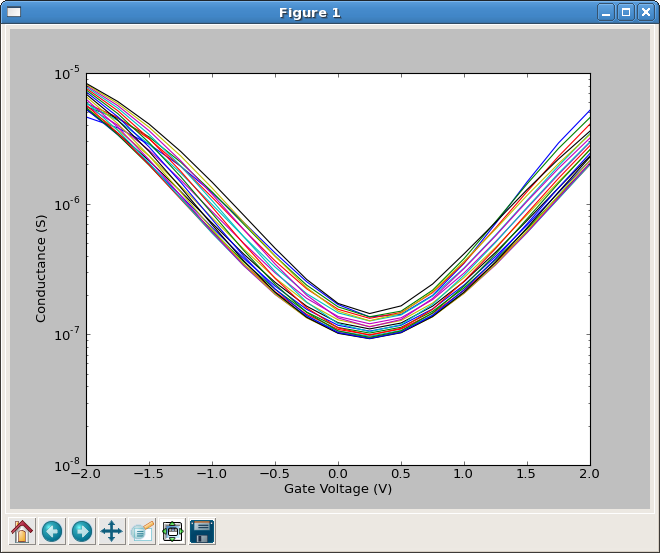
Fig. 88 Conductance as a function of the gate potential. Different curves are for different electron temperatures, namely 0, 100, 200, …, 2000 Kelvin.

The conductance has a minimum for a gate potential of about 0.25 Volt. At this point, the Fermi level is positioned in the mid gap between the valence and conductance band of the central ribbon. Note that there is only a weak dependence of the conductance on the electron temperature, which illustrates that the transmission is dominated by electron tunnelling.

Tip

This tutorial relies heavily on scripting access to inputs and outputs of the TransmissionSpectrum object. For further information on all the options and methods available, see the ATK Reference Manual.

Also note that we use the pylab package to generate plots. This is readily available with atkpython and is very handy for making plots with Python scripts.

Linear response calculations

You just saw that the transmission spectra for different gate potentials are rather similar and that the main difference is a shift of the band edges relative to the Fermi level. This suggests that you may avoid the self-consistent loop and simply shift the Fermi level rigidly and calculate all the transmission spectra using linear response theory.

The following script implements a linear response calculation of the conductance as function of the gate potential, assuming that the effect of the gate potential is a simple shift of the relative positions of the electrode Fermi levels within the transmission spectra. You can download it here: linear_response.py.

#make list of relevant temperatures
temperature_list=numpy.linspace(0,2000,21)*Kelvin
#make list of relevant gate voltages
gate_voltage_list=numpy.linspace(-2.0,2.0,17)*Volt
#make list to hold the conductance calculations
conductance_list=numpy.zeros(len(gate_voltage_list)*len(temperature_list))
conductance_list=conductance_list.reshape(len(gate_voltage_list),
                                          len(temperature_list))
#read the reference transmission spectrum from the netcdf data file
gate_potential_ref = 0.*Volt
transmission_spectrum = nlread("gatescan-6-6.nc",
    object_id="trans"+str(gate_potential_ref))[0]
#loop through the gate voltages
for n in range(len(gate_voltage_list)):
    #loop through the temperature list
    for i in range(len(temperature_list)):
        conductance_list[n,i]=transmission_spectrum.conductance(
            electrode_temperatures=(temperature_list[i],temperature_list[i]),
            electrode_voltages=(gate_voltage_list[n]-gate_potential_ref,
                                gate_voltage_list[n]-gate_potential_ref))
#plot the conductance as function of gatevoltage
import pylab
pylab.figure()
# make curve for each temperature
for i in range(len(temperature_list)):
    pylab.semilogy(gate_voltage_list,conductance_list[:,i])
pylab.xlabel("Gate Voltage (V)")
pylab.ylabel("Conductance (S)")
pylab.show()

The script implements a quite simple workflow:

1. It reads in the transmission spectrum from the calculation with 0 V gate potential:

#read the reference transmission spectrum from the netcdf data file
gate_potential_ref = 0.*Volt
transmission_spectrum = nlread("gatescan-6-6.nc",
    object_id="trans"+str(gate_potential_ref))[0]

2. Instead of setting the gate potential, the electrode voltages are varied such that the electrode Fermi levels are shifted relative to each other:

            electrode_voltages=(gate_voltage_list[n]-gate_potential_ref,
                                gate_voltage_list[n]-gate_potential_ref))

The script produces the figure below. We see that the main main trends of the fully self-consistent calculations are reproduced by the linear response procedure.

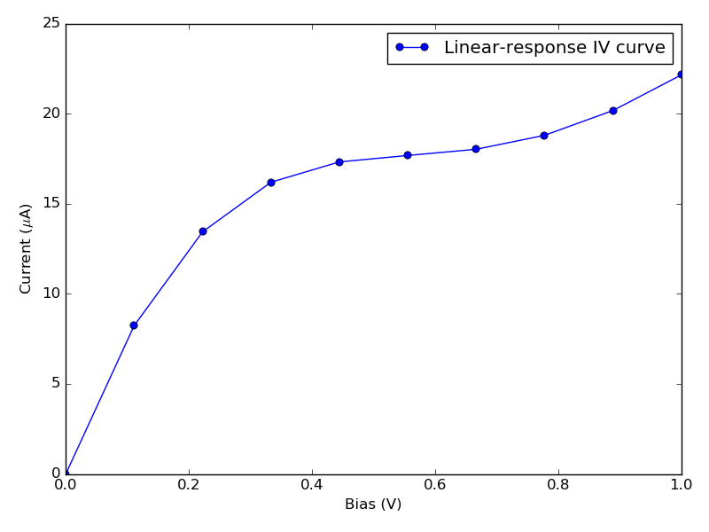
Fig. 89 Conductance as function of the gate potential calculated using linear response. Different curves are for electron temperatures 0, 100, 200, …, 2000 Kelvin.

I–V characteristics

You will now investigate the effect of changing the external bias across the electrodes in the range 0-2 Volt. The calculations follow a similar procedure as the gate potential scan in the previous section.

Electrode bias loop

Use the script displayed below. You can download it here: electrode_loop.py.

# Read in the old configuration
device_configuration = nlread("z-a-z-6-6.nc",DeviceConfiguration)[0]
calculator = device_configuration.calculator()
# Output filename
filename = 'ivscan-6-6.nc'
# Define bias voltages
voltage_list=numpy.linspace(0.0,2.0,9)*Volt
for voltage in voltage_list:
    # Set new calculator with modified electrode voltages on the configuration
    # use the self consistent state of the old calculation as starting input.
    device_configuration.setCalculator(
    calculator(electrode_voltages=(-0.5*voltage,0.5*voltage)),
               initial_state=device_configuration)
    #Analysis
    electron_density = ElectronDifferenceDensity(device_configuration)
    nlsave(filename, electron_density, object_id='dens'+str(voltage))
    electrostatic_potential = ElectrostaticDifferencePotential(device_configuration)
    nlsave(filename, electrostatic_potential, object_id='pot'+str(voltage))
    transmission_spectrum = TransmissionSpectrum(
        configuration=device_configuration,
        energies=numpy.linspace(-2,2,200)*eV)
    nlsave(filename, transmission_spectrum, object_id='trans'+str(voltage))
    nlprint(transmission_spectrum)

The calculation uses the calculation for the junction with an applied gate potential of -1 V as a starting point. This value for the gate potential is fixed through the entire calculation. The electrode voltages are modified through the electrode_voltages variable of the DeviceHuckelCalculator.

The entire calculation will take more than 10 times longer than the single zero bias calculation. During the loop, the results will be saved in the file ivscan-6-6.hdf5. The file may be inspected during the calculation to follow how the calculation is progressing.

The plot below shows the electrostatic potential for a bias of 1 Volt, i.e. -0.5 V on the left electrode and +0.5 V on the right electrode. Notice how the electrostatic potential in the left electrode is closer to the electro-static potential of the gate.

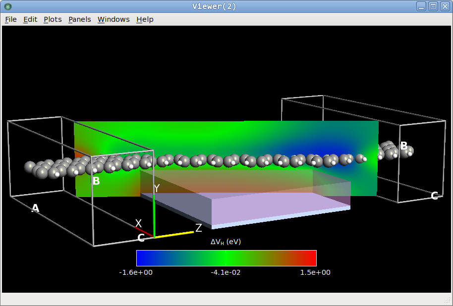
Fig. 90 Electrostatic potential of the junction with a symmetrically applied bias of 1 Volt and a gate potential of -1 Volt.

Self-consistent I–V characteristics

You can now use all the TransmissionSpectrum objects in ivscan-6-6.hdf5 to calculate the I–V curve for a gate potential of -1 V. Use the script shown below, which combines the methods presented in the previous sections. You can also download it here: IV_curve.py.

#make list of relevant temperatures
temperature_list=numpy.linspace(0,2000,21)*Kelvin
#make list of relevant gate voltages
voltage_list=numpy.linspace(0.0,2.0,9)*Volt
#make list to hold the current calculations
current_list=numpy.zeros(len(voltage_list)*len(temperature_list))
current_list=current_list.reshape(len(voltage_list),len(temperature_list))
#specify the filename for the netcdf data file
filename="ivscan-6-6.nc"
#loop through the gate voltages
for n in range(len(voltage_list)):
    transmission_spectrum=nlread(filename, object_id="trans"+str(voltage_list[n]))[0]
    #loop through the temperature list
    for i in range(len(temperature_list)):
        current_list[n,i]=transmission_spectrum.current(
            electrode_temperatures=(temperature_list[i],temperature_list[i]))
#plot the current as function of voltage
import pylab
pylab.figure()
# make curve for each temperature
for i in range(len(temperature_list)):
    pylab.plot(voltage_list,current_list[:,i])
pylab.xlabel("Bias (V)")
pylab.ylabel("Current (A)")
pylab.show()

The result of the calculation is illustrated below.

Fig. 91 Self-consistent current-voltage characteristics of the nanoribbon junction with -1 V gate potential. Curves are for electrode temperatures 0, 100, 200, .. 2000 Kelvin. The electric current increases with temperature.

Linear response I–V characteristics

Similar to the linear response approximation for the gate potential presented in the previous section, you may use a linear response approximation to calculate the finite-bias transmission spectra from the zero-bias spectrum. The following script performs a calculation of the linear response current for an electrode temperature of 300 Kelvin:

#make list of relevant temperatures
temperature=300*Kelvin
#make list of relevant gate voltages
voltage_list=numpy.linspace(0.0,2.0,9)*Volt
#make list to hold the current calculations
current_list=numpy.zeros(len(voltage_list))
current_list_lin=numpy.zeros(len(voltage_list))
#read the reference transmission spectrum from the netcdf data file
potential_ref = 0.*Volt
filename="ivscan-6-6.nc"
transmission_spectrum0 = nlread(filename, object_id="trans"+str(potential_ref))[0]
for n in range(len(voltage_list)):
    transmission_spectrum=nlread(filename, object_id="trans"+str(voltage_list[n]))[0]
    current_list[n]=transmission_spectrum.current(
        electrode_temperatures=(temperature,temperature))
    current_list_lin[n]=transmission_spectrum0.current(
        electrode_temperatures=(temperature,temperature),
        electrode_voltages=(-0.5*(voltage_list[n]-potential_ref),
        0.5*(voltage_list[n]-potential_ref) ) )
#plot the current as function of bias
import pylab
pylab.figure()
pylab.plot(voltage_list,current_list,label="self consistent")
pylab.plot(voltage_list,current_list_lin,label="linear response")
pylab.xlabel("Bias (V)")
pylab.ylabel("Current (A)")
pylab.legend(loc="lower left")
pylab.grid(True)
pylab.show()

The figure below compres the linear response results to the self-consistent ones. The agreement is quite good for low bias, but at large bias the linear response current does start to deviate from the self-consistently calculated current.

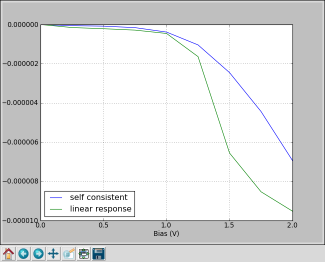
Fig. 92 Comparison of the self-consistent (blue) and linear response (green) current-voltage characteristics of the junction with a -1 V gate potential and an electrode temperature of 300 Kelvin.

When is the linear response approximation valid?

The previous sections illustrate how to perform calculations of the current as function of the electrode bias or the gate potential. Even though the methodology is based on the extended Huckel formalism, such calculations can be quite time consuming, and an alternative is to invoke the linear response approximation in and use non-self-consistent calculations, which are much faster than self-consistent ones.

However, an important question emerges: When is it OK to use linear response instead of fully self-consistent calculations? You have already seen that linear response works well for a relatively small electrode bias, but how about the influence of the gate potential?

The scripts presented in the previous sections can be easily modified to vary the gate potential and the electrode bias simultaneously. Below is a comparison between the self-consistent current and the linear response current. For a small bias and gate potential the two are in good agreement, illustrating that the linear response current is a good first approximation.

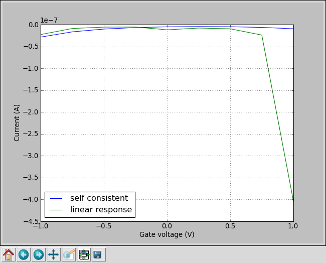
Fig. 93 Current for an applied bias of 0.2 Volt as a function of the gate potential. The blue curve was obtained from a fully self-consistent calculation, while the green curve was obtained from a linear response calculation using the transmission spectrum of a system with zero gate potential and bias.

The scripts that generated the self-consistent data at the plot can be downloaded here: potentials_vary.py, electrode_0.2V_gate_varies.py.

Further analysis with ATK-SE

Some of the other analyses that can be performed with QuantumATK are

• 3D visualization of scattering states.

• 3D visualization of transmission pathways.

• Projected density of states.

The main part of the analysis in this tutorial are performed using QuantumATK scripts. However, analysis can in most cases also be performed directly from the QuantumATK GUI. For further information, see the Transport calculations with QuantumATK.

Temperature dependent conductance

In this section you will learn how the transmission spectrum can be used to calculate the conductance of the device as a function of the left and right electrode temperatures, \(T_L\) and \(T_R\). At \(T_L=T_R=0\), the conductance is determined by the transmission coefficient at the Fermi Level, while for finite electrode temperatures, the conductance depends on the value of the transmission coefficient in an energy window around the Fermi level. The zero-bias conductance is given by

\[\sigma (T_L)=\frac{2e^2}{h}\int T(E) \; f^\prime (\eta(E)) \frac{dE}{k_bT_R},\]

where \(f^\prime (\eta(E)) = f^\prime \left(\frac{E-E_F^L}{k_bT_R}\right)\) is the derivative of the Fermi function [2].

In semiconductors the conductance is often determined by hot electrons or holes propagating within the conduction or valence band, so-called thermionic emission. The hot electrons are located in the energy range of the tails of the Fermi function. Thus, for an accurate calculation of the conductance from thermionic emission, it is important that the energy range of the transmission spectrum is such that the tails of the Fermi functions are properly sampled. The transmission spectrum figure in the previous chapter shows that both the valence and conduction band edges of the central region are within the energy range of the transmission spectrum. From that data you will therefore be able to accurately determine the temperature dependent conductance.

Use the following QuantumATK script to calculate and plot the temperature dependent conductance. It can be downloaded here: temperature_dependent.py.

# Read first transmission spectrum from file z-a-z-6-6.hdf5
transmission_spectrum = nlread("z-a-z-6-6.hdf5",TransmissionSpectrum)[0]
#make list of temperatures
temperature_list=numpy.linspace(0,2000,21)*Kelvin
#make list for holding conductance
conductance_list=numpy.zeros(len(temperature_list))
#calculate the conductance for each temperature in the temperature list
for i in range(len(temperature_list)):
    conductance_list[i]=transmission_spectrum.conductance(
        electrode_temperatures=(temperature_list[i], temperature_list[i]))
#plot the conductance as function of temperature
import pylab
pylab.figure()
pylab.semilogy(temperature_list,conductance_list)
pylab.xlabel("Temperature (K)")
pylab.ylabel("Conductance (S)")
pylab.show()

The script reads the previously calculated transmission spectrum and then uses the conductance() method for calculating the conductance for a number of electrode temperatures. Save the script and run it using the Job Manager or run it from a terminal:

$ atkpython temperature_dependent.py

You will obtain the figure below.

The temperature dependent conductance for this device is typical for a field effect transistor: The initial decrease in conductance as a function of temperature is related to a large conductance at the Fermi level caused by electron tunneling. At larger temperatures, the usual increase of conductance with temperature starts dominating. The tunneling effect will be suppressed in a longer device, as you will see in the next section.

Comparison to results for a longer device

Attention

This section employs a device with a longer nanoribbon. Build the device as described here: A longer nanoribbon transistor.

You will now calculate the transmission spectrum of the nanoribbon transistor with a longer channel, and compare its temperature dependent conductance with the shorter system investigated earlier.

Electron conductance

Open the large transistor configuration in the Builder, and confirm that it looks as expected. Next step is to set up the calculations needed for analyis of the electronic conductance in exactly the same way as outlined in the previous section for the shorter device. There are two ways to do this:

1. Send the device to the Scripter and repeat all the steps that were needed to prepare the script z-a-z-6-6.py, and save the new script as z-a-z-20-6.py.

2. Alternatively, you may use the Editor to generate the new script:

   • Save the new geometry into the file z-a-z-20-6.py.

   • Copy the lines specifying the calculation from z-a-z-6-6.py, and insert them into z-a-z-20-6.py.

Note

Remember to change the HDF5 output filename to z-a-z-20-6.hdf5.

• The part of the script specifying the calculation is found below the lines indicating “Calculator”:

######################################################
# Calculator
######################################################

• Run the script using the Job Manager or from a terminal. The calculation will take approximately twice as much time as the previous calculation for the shorter junction.

• When the calculation is done, use the script below to plot and compare the temperature dependent conductance of the two junctions. You can download it here: temperature_dependent_compare.py.

# Read first transmission spectra from fil z-a-z-6-6.hdf5 and z-a-z-20-6.hdf5
transmission_spectrum6 = nlread("z-a-z-6-6.hdf5",TransmissionSpectrum)[0]
transmission_spectrum20 = nlread("z-a-z-20-6.hdf5",TransmissionSpectrum)[0]
#make list of temperatures
temperature_list=numpy.linspace(0,2000,21)*Kelvin
#make list for holding conductance
conductance_list6=numpy.zeros(len(temperature_list))
conductance_list20=numpy.zeros(len(temperature_list))
for i in range(len(temperature_list)):
    conductance_list6[i]=transmission_spectrum6.conductance(
        electrode_temperatures=(temperature_list[i],temperature_list[i]) )
    conductance_list20[i]=transmission_spectrum20.conductance(
        electrode_temperatures=(temperature_list[i],temperature_list[i]) )
#plot the conductance as function of temperature
import pylab
pylab.figure()
pylab.semilogy(temperature_list,conductance_list6,label="short junction")
pylab.semilogy(temperature_list,conductance_list20,label="long junction")
pylab.xlabel("Temperature (K)")
pylab.ylabel("Conductance (S)")
pylab.legend(loc="lower left")
pylab.grid(True)
pylab.show()

Below is the result of the calculation. The green curve shows the result for the longer junction. Note that in this case the conductance increases strongly with temperature, indicating that the dominating transport mechanism is thermionic emission rather than electron tunneling.

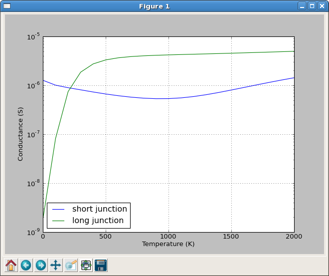
Fig. 94 Conductance as a function of the electron temperature for the short (blue) and 20 unit long (green) graphene nanoribbon transistor.

Electron thermal transport

In the previous section you calculated the conductance of the junction. To obtain an electrical current it is usually necessary to apply an external bias. This section shows how it is also possible to drive a current through the junction by having the two electrodes at different temperatures. The QuantumATK script for the calculation is displayed below. You can download the script here: electrodes_diff_temperature.py.

# Read first transmission spectra from file z-a-z-6-6.hdf5 and z-a-z-20-6.hdf5
transmission_spectrum6 = nlread("z-a-z-6-6.hdf5",TransmissionSpectrum)[0]
transmission_spectrum20 = nlread("z-a-z-20-6.hdf5",TransmissionSpectrum)[0]
#make list of temperatures
temperature_list=numpy.linspace(0,2000,21)*Kelvin
#make list for holding current
current_list6=numpy.zeros(len(temperature_list))
current_list20=numpy.zeros(len(temperature_list))
#fix the temperature in the left electrode
temperature_left=300*Kelvin
for i in range(len(temperature_list)):
    current_list6[i]=transmission_spectrum6.current(
        electrode_temperatures=(temperature_left,temperature_list[i]) )
    current_list20[i]=transmission_spectrum20.current(
        electrode_temperatures=(temperature_left,temperature_list[i]) )
#plot the current as function of temperature in right electrode
import pylab
pylab.figure()
pylab.plot(temperature_list,current_list6,label="short junction")
pylab.plot(temperature_list,current_list20,label="long junction")
pylab.xlabel("Right Electrode Temperature (K)")
pylab.ylabel("Current (A)")
pylab.legend(loc="lower left")
pylab.grid(True)
pylab.show()

The electron temperature of the left electrode is now fixed at 300 Kelvin, while the temperature of the right electrode is varied from 0 to 2000 Kelvin. The figure below shows the output of the calculation. The change in temperature has the strongest effect on the longer junction (the green curve). The positive direction of the current is from left to right, thus, the electrical current goes from the high temperature to the low temperature.

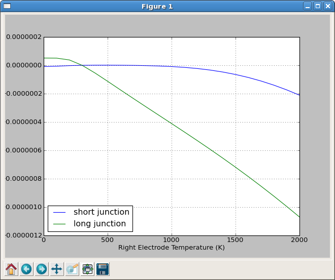
Fig. 95 Current as a function of the electron temperature of the right electrode for the short (blue) and 20 unit long (green) graphene junction. The electron temperature of the left electrode is fixed at 300 Kelvin.

If you use the Transmission Analyzer to plot the transmission spectrum for the long junction, you will see that the valence band of the central region is closest to the Fermi Level. The charge transport is therefore dominated by hole transport. The electrode with the highest temperature will have most holes, which will propagate to the other electrode, giving rise to a current in this direction.

References

[1]

J. Cerda and F. Soria. Accurate and transferable extended Hückel-type tight-binding parameters. Phys. Rev. B, 61:7965–7971, Mar 2000. doi:10.1103/PhysRevB.61.7965.

[2]

H. H. B. Sorensen, P. C. Hansen, D. E. Petersen, S. Skelboe, and K. Stokbro. Efficient wave-function matching approach for quantum transport calculations. Phys. Rev. B, 79:205322, May 2009. doi:10.1103/PhysRevB.79.205322.