Spin transport in magnetic tunnel junctions
Version: 2016.0
Introduction
This tutorial shows you how to simulate and analyze the electronic transport properties of magnetic tunnel junctions (MTJs), commonly studied for spintronic applications. You will consider a Fe|MgO|Fe MTJ, which is a rather complex spin polarized system, initially studied by MacLaren and co-workers [1].
You will use QuantumATK to study the colinear and non-colinear spin-dependent transport properties, including electronic transmission, tunnel magnetoresistance, and spin-transfer torque. You will also become acquainted with the AdaptiveGrid method, which is an adaptive alternative to the conventional Monkhorst–Pack type grid for k-point sampling.

Getting started
It is very easy to create a Fe|MgO|Fe tunnel junction using the Magnetic Tunnel
Junction Builder plugin. However, the device configuration will then need to be
geometry optimized, which is not the main objective of this tutorial. We therefore
provide an QuantumATK Python script with the optimized device central region, central_region.py,
which you should use for building the MTJ device. You can also jump to section
Relaxing the device central region if you want to learn how the geometry relaxation was done.
For now, just start QuantumATK, create a new project and give it a name, then select it
and click Open. Download central_region.py and save it in the Project Folder. Then drop
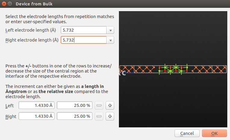
the script on the QuantumATK  Builder, and use the Device from Bulk
plugin to attach electrodes to the central region, and thereby create the Fe|MgO|Fe
device.
Builder, and use the Device from Bulk
plugin to attach electrodes to the central region, and thereby create the Fe|MgO|Fe
device.
The default electrode length of 5.732 Å will work fine for the present purposes. This corresponds to two times the iron lattice constant.
Note
The Device from Bulk plugin will suggest a few different electrode lengths. These are detected by searching for periodicity in your central region. Always check and carefully choose these important parameters. See the tutorial Transport calculations with QuantumATK for more information.
Parallel spin
You will in the following perform a self-consistent NEGF-DFT calculation for the case of parallel spin polarization in the left and right iron parts of the MTJ. You will also compute the transmission spectrum as a function of the k-vector parallel to the transport direction.
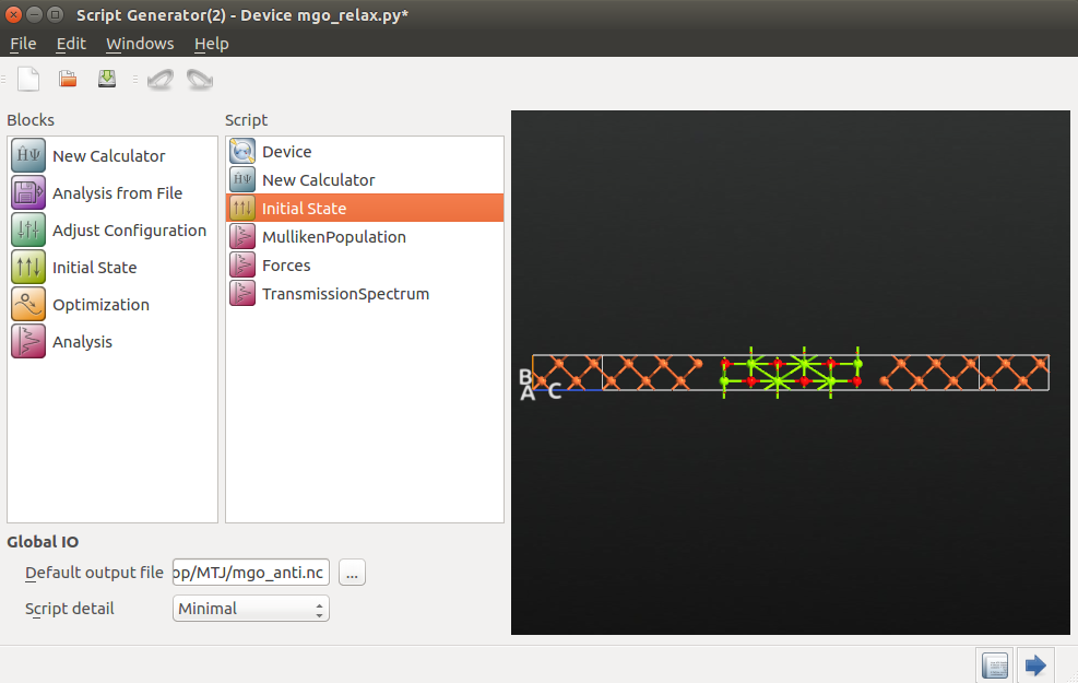
Send the device configuration to the  Script Generator
(use the
Script Generator
(use the  icon for this), and add the following blocks to the script:
 New Calculator
 Initial State
 MullikenPopulation
- Forces
- TransmissionSpectrum
Then change the default output file name to mgo_para.nc.

Next, adjust the settings in a some of the script blocks:
Calculator:
Select the SGGA exchange-correlation method, to perform a spin polarized GGA calculation using the PBE functional.
Increase the electron temperature to 1200 Kelvin, to ease the self-consistent convergence.
Use a 7x7x100 k-point grid.
Select the SingleZetaPolarized basis set for iron.
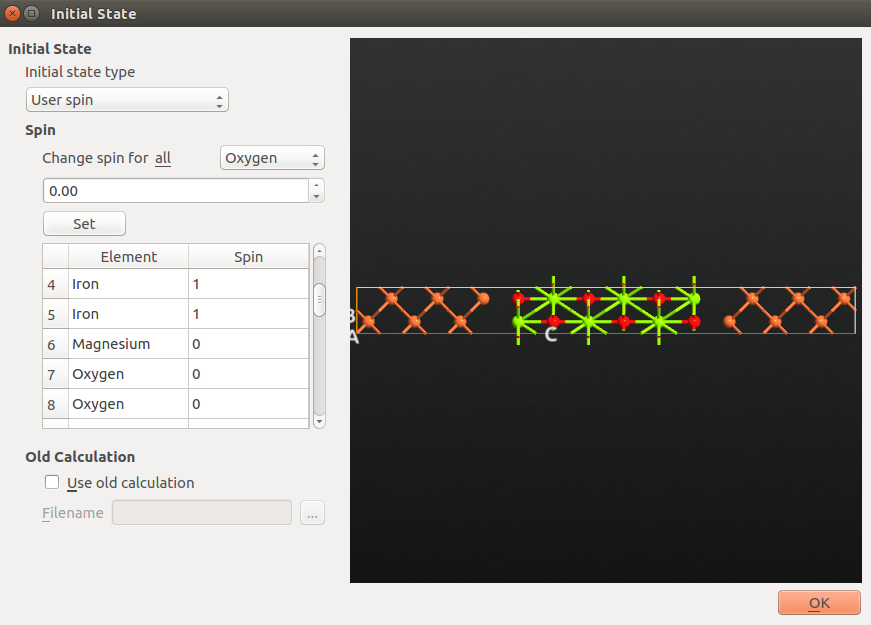
Initial State:
Choose User spin for as the type of initial state.
Set the relative spins on O and Mg atoms to 0.
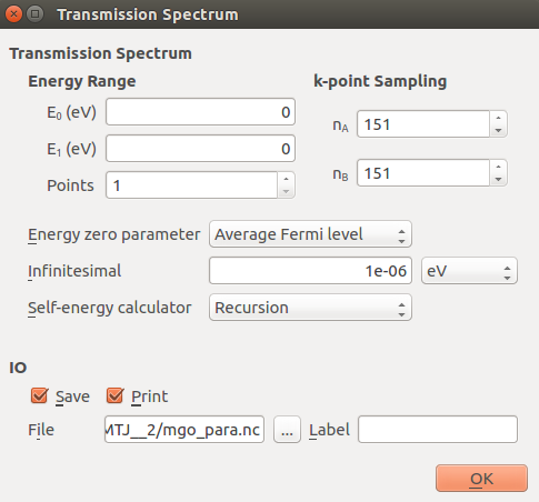
TransmissionSpectrum:
You will in this example compute the transmission only at the Fermi level, to save time. Use the settings E0 = E1 = 0.0 eV and just a single energy point to achieve this.
151x151 grid for k-point sampling.
Save the script as mgo_para.py and run the calculation, e.g. using the
 Job Manager. The calculations may take an hour on a single
core, but it is possible to obtain a very good speedup by executing in parallel,
reducing the computational time down to roughly 20 minutes with 4 MPI processes.
If needed you can also download the script:
Job Manager. The calculations may take an hour on a single
core, but it is possible to obtain a very good speedup by executing in parallel,
reducing the computational time down to roughly 20 minutes with 4 MPI processes.
If needed you can also download the script: mgo_para.py.
Important
Do not close the Script Generator window. You will need it again later on for setting up calculations for the anti-parallel spin configuration.
Inspecting the forces
The output data file mgo_para.nc should now have appeared in the Project
Files list. Make sure it is selected, such that the data items are visible on the
LabFloor. Then select the Forces item and use the Text Representation tool
in the right-hand Panel Bar to see a report of the forces:
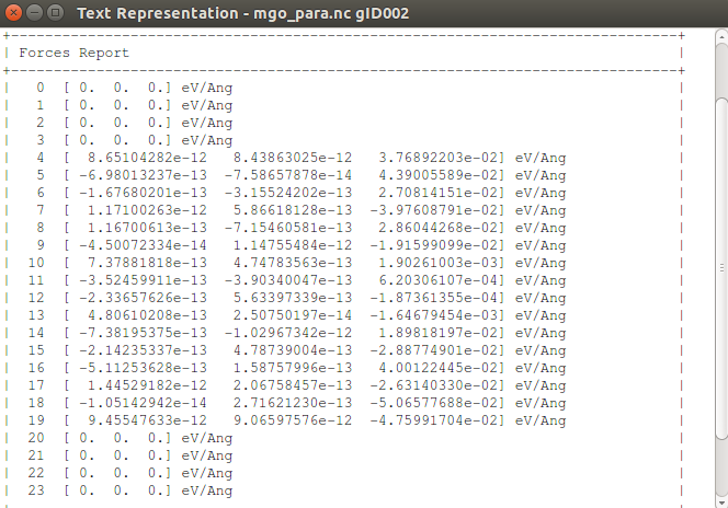
The forces on the atoms belonging to the electrode extension regions are not calculated, and these are therefore set to zero. For the other atoms, the forces are small.
Mulliken population
You can also use the Text Representation tool to inspect the calculated Mulliken populations:
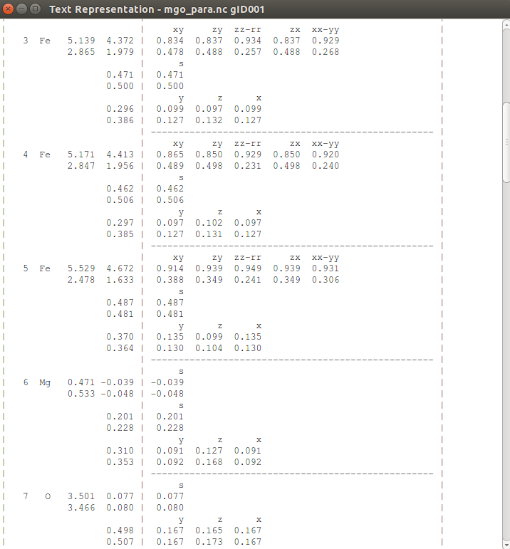
The leftmost column lists the total Mulliken population per spin channel for each atom. It is important to inspect this result in order to check that each atom is correctly spin polarized. Note that all Fe atoms are polarized with their majority spin pointing up, while the O atoms are essentially unpolarized. The Mg atoms next to the interfaces (on both sides) couple anti-parallel with the Fe atoms, while the Mg atoms further away from the interfaces are unpolarized.
The report also shows the population for each shell and resolves it on individual orbitals.
Electron transmission
Use the Transmission Analyzer plugin to analyze the calculated transmission spectrum. A few modifications of the plotting options make this spectrum easier to analyze:
Right-click the right-hand plot of the k-dependent transmission coefficients, and select the color map named Spectral.
In the Curves menu, tick off Up and Down.
Using the Active Spin menu, you can now choose between the k-dependent transmission for spin-up and spin-down electrons:

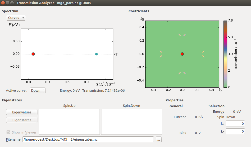
As for the results of the calculation, it is clear from the plots above that the spin-down (minority) transmission is strongly suppressed in magnitude, and exhibits spikes at certain points in the Brillouin zone, corresponding to resonant tunneling, whereas the spin-up (majority) transmission indicates regular barrier tunneling. This is all in agreement with the accepted picture of the tunneling mechanism in the Fe|MgO|Fe tunneling junction (compare to Figures 6 and 10 in [1]).
Anti-parallel spin
We now turn to the case of anti-parallel alignment of the spins in the left and right iron parts of the Fe|MgO|Fe junction. The self-consistent state of the parallel configuration computed above will be used as an initial guess for the anti-parallel state. This speeds up SCF convergence as compared to starting the anti-parallel calculation completely from scratch.
Return to the Script Generator. If you did not close
it after setting up the parallel calculation, only a few modifications are needed.
Otherwise, drop the script mgo_para.py on the Scripter and start by setting
up the script identically to what you did above for the parallel calculations.
Setting the initial state
Open the Initial State block, and do the following to set up
the anti-parallel spin configuration and use the parallel calculation as an initial
guess for the device density matrix:
Set again the relative spin for all iron atoms to 1 and set it to 0 for magnesium and oxygen atoms.
Change the initial spin to -1 for all iron atoms on the right-hand side of the junction.
Check the Use old calculation tick box and enter
mgo_para.ncas the filename from which the old calculation should be loaded from.

Note
The method ouitlined above works like this: The converged density matrix from the parallel-spin calculation is used as initial state. However, the spin densities for atoms in the right-hand side of the device are flipped, resulting in an anti-parallel initial density matrix for the full device.
Finally, change the default output file name to mgo_anti.nc and make sure
the TransmissionSpectrum analysis block is identical to the one used for the
spin-parallel case.
Save the QuantumATK Python script as mgo_anti.py and run it.
Analyzing the results
Check that the forces on each atom are still negligible. Also check the Mulliken populations to ensure that each atom has the expected spin polarization.
Use again the Transmission Analyzer to analyze the electronic transmission. In this case, the transmission for up and down (majority and minority) spins are identical because of the mirror symmetry of the system. We find again that the k-dpendent transmission coefficients exhibit highly localized peaks surrounded by regions of zero transmission.
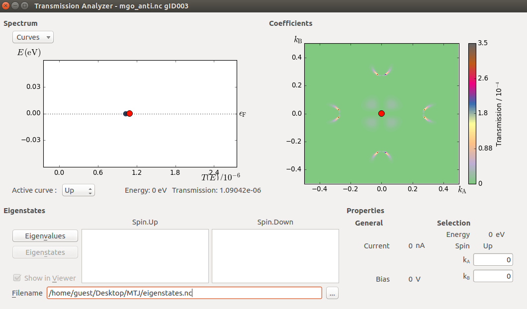
To understand why the transmission is identical for spin-up and -down, first note that due to time inversion symmetry, propagation from left to right is always identical to propagation from right to left. The “up” component of the transmission spectrum corresponds to “up” electrons from the left electrode propagation into the right electrode. The “down” component of the transmission spectrum corresponds to “down” electrons in the right electrode propagating into the left electrode.
Due to the anti-symmetric spin, the up electrons in the left electrode and the down electrons in the right electrode are both majority channels. Because of the mirror symmetry of the device, the propagation of the left majority channels into the right minority channels (the first transmission coefficient spin component) and the propagation of the right majority channels into the left minority channels (the second transmission coefficient spin component) are the same.
Thus, for symmetric devices, the equivalence of the two spin channels is an important check for anti-symmetric calculations at zero bias.
Tunneling magnetoresistance
The tunneling magnetoresistance (TMR) is defined as
where \(G_P\) is the conductance through the junction with parallel spin alignment and \(G_{AP}\) the conductance for anti-parallel spin alignment.
The conductances can be calculated from their respective transmission spectra.
The script below performs this calculation. You can download it here: tmr.py.
# Calculate conductance for parallel spin
transmission_para = nlread('mgo_para.hdf5', TransmissionSpectrum)[0]
conductance_para_uu = transmission_para.conductance(spin=Spin.Up)
conductance_para_dd = transmission_para.conductance(spin=Spin.Down)
conductance_para = conductance_para_uu + conductance_para_dd

# Calculate conductance for anti-parallel spin
transmission_anti = nlread('mgo_anti.hdf5', TransmissionSpectrum)[0]
conductance_anti_uu = transmission_anti.conductance(spin=Spin.Up)
conductance_anti_dd = transmission_anti.conductance(spin=Spin.Down)
conductance_anti = conductance_anti_uu + conductance_anti_dd

print('Conductance Parallel Spin (Siemens)')
print('Up=%8.2e, Down=%8.2e' % (conductance_para_uu.inUnitsOf(Siemens),
                                conductance_para_dd.inUnitsOf(Siemens)))
print('Total = %8.2e' % (conductance_para.inUnitsOf(Siemens)))
print()

print('Conductance Anti-Parallel Spin (Siemens)')
print('Up=%8.2e, Down=%8.2e' % (conductance_anti_uu.inUnitsOf(Siemens),
                                conductance_anti_dd.inUnitsOf(Siemens)))
print('Total = %8.2e' % (conductance_anti.inUnitsOf(Siemens)))
print()

print('TMR (optimistic)  = %8.2f percent' % \
      (100.*(conductance_para-conductance_anti)/conductance_anti))
print('TMR (pessimistic) = %8.2f percent' % \
      (100.*(conductance_para-conductance_anti)/(conductance_para+conductance_anti)))
Execute the script, and find the TMR:
Conductance Parallel Spin (Siemens)
Up=4.11e-09, Down=2.79e-10
Total = 4.39e-09

Conductance Anti-Parallel Spin (Siemens)
Up=4.22e-11, Down=4.00e-11
Total = 8.22e-11

TMR (optimistic)  =  5240.12 percent
TMR (pessimistic) =    96.32 percent
Adaptive k-point grid
The AdaptiveGrid class implements an alternative to the traditional Monkhorst–Pack
(MP) grid for k-point sampling. As described in great detail in the QuantumATK Reference Manual
entry for AdaptiveGrid, an adaptive k-point grid can be used to automatically
zoom in on the significant features of the electron transmission spectrum. This is
particularly useful when the k-dependent transmission is dominated by localized peaks,
like for the Fe|MgO|Fe MTJ, where the total computed transmission may depend critically
on resolving those peaks.
The adaptive algorithm essentially divides the Brillouin zone (BZ) into triangles and
integrates over each triangle. Each triangle becomes increasingly small in an
iterative manner until convergence is reached, but stops if the number of refinement
levels reach the maximum_number_of_levels, which is 20 by default. Two types of
error measures are available:
- Absolute:
Converged when the absolute value of the BZ integral in all triangles is lower than the chosen tolerance.
- Relative:
Converged when the relative value of the BZ integral in all triangles is lower than the chosen tolerance.
Note
The AdaptiveGrid functionality is available from QuantumATK 2016 an onwards.
The figures below show how the total transmission through the Fe|MgO|Fe MTJ depends on the k-point resolution used for sampling the k-dependent transmission function for the parallel and anti-parallel cases. Results using the MP k-point grid are compared to those from using the adaptive k-point grid.
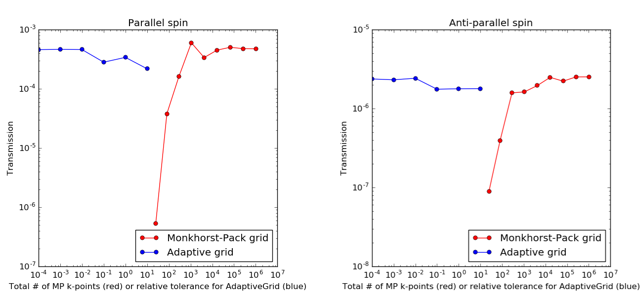
Well converged calculations of the total transmission through the MTJ considered here are obtained with no less than 103 Monkhorst–Pack k-points, roughly corresponding to a 31x31 grid. With the adaptive k-point grid, a relative tolerance of 10-2 seems to be quite sufficient.
Note
The computational load for producing the data shown in the figures above increase from right to left with AdaptiveGrid (blue curves), and from left to right with MonkhorstPack (red curves).
Parallel transmission
The script adaptive_grid.py calculates the transmission for the Fe|MgO|Fe device with
parallel spin orientation using both a dense MP grid and the AdaptiveGrid method:
# -------------------------------------------------------------
# Load device configuration
# -------------------------------------------------------------
device_configuration = nlread('mgo_para.nc', DeviceConfiguration)[0]

# -------------------------------------------------------------
# Transmission Spectrum using a dense Monkhorst-Pack grid.
# -------------------------------------------------------------
transmission_spectrum = TransmissionSpectrum(
    configuration=device_configuration,
    energies=numpy.linspace(0,0,1)*eV,
    kpoints=MonkhorstPackGrid(500,500),
    )
nlsave('adaptive_grid.nc', transmission_spectrum)

# -------------------------------------------------------------
# AdaptiveGrid.
# -------------------------------------------------------------
adaptive_grid = AdaptiveGrid(
    tolerance=0.01,
    error_measure=Relative)

# -------------------------------------------------------------
# Transmission Spectrum using the AdaptiveGrid.
# -------------------------------------------------------------
transmission_spectrum = TransmissionSpectrum(
    configuration=device_configuration,
    energies=numpy.linspace(0,0,1)*eV,
    kpoints=adaptive_grid,
    )
nlsave('adaptive_grid.nc', transmission_spectrum)
The Monkhorst–Pack grid has 500x500 k-points, while the adaptive grid is set up with a relative tolerance of 10-2. Download and run the script. It should finish in roughly 25 minutes if executed in parallel with 4 MPI processes on a modern laptop.
Spin-up transmission

Fig. 113 Spin-up transmission spectrum evaluated using a 500x500 Monkhorst–Pack grid. The total k-point averaged spin-up transmission is 4.6 \(\cdot\)10-4. Left: Full BZ view. Right: Zoom-in around the Г point.
The spin-up spectrum obtained with the dense Monkhorst–Pack grid is different from the one obtained in section Electron transmission using a less dense grid: We now see that the feature in the middle of the spectrum is actually circular, with zero transmission immediately around the Г point. Clearly, a very dense grid is needed to resolve this fact. Note, however, that the improved k-point sampling has only increased the total k-point averaged spin-up transmission by a factor of 4.
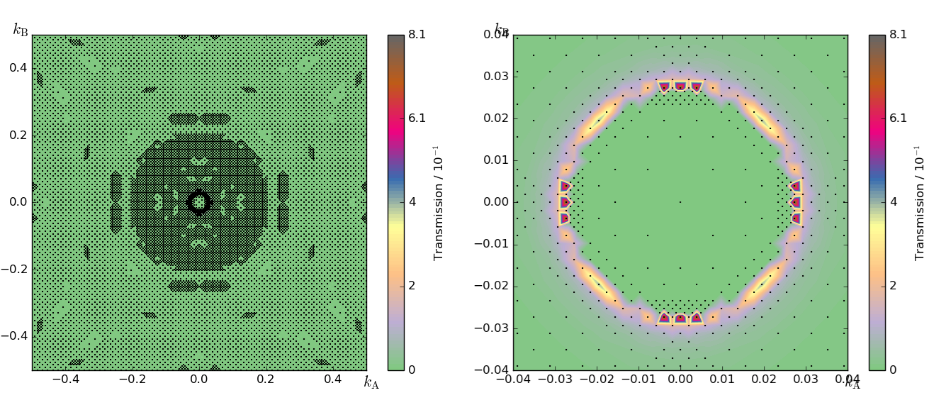
Fig. 114 Spin-up transmission spectrum evaluated using an adaptive grid using a relative tolerance of 10-2. The black dots indicate the sampled k-points. The total k-point averaged spin-up transmission is 4.2 \(\cdot\)10-4. Left: Full BZ view. Right: Zoom-in around the Г point.
The spin-up transmission spectrum evaluated using an adaptive grid is shown in the figure above, where the black dots indicate the sampled k-points. The adaptive algorithm has clearly zoomed in on the circular feature of the k-dependent transmission, causing the k-point density to be largest around the circular transmission feature.
Spin-down transmission
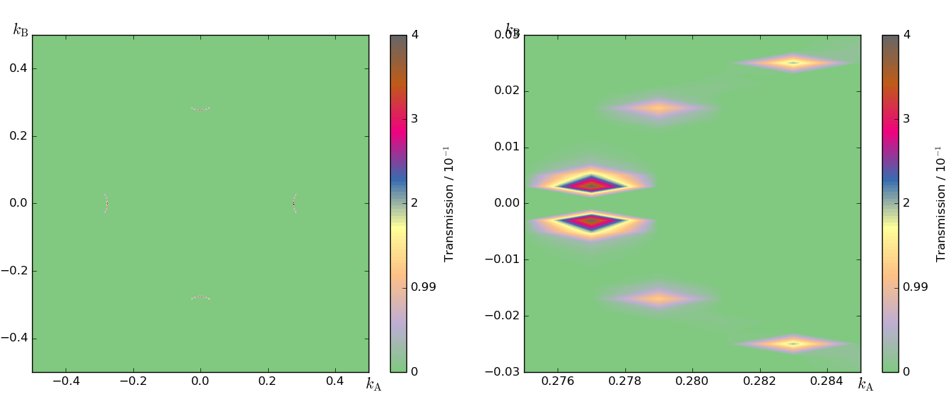
Fig. 115 Spin-down transmission spectrum evaluated using a 500x500 Monkhorst–Pack grid. The total k-point averaged spin-down transmission is 3.7 \(\cdot\)10-5. Left: Full BZ view. Right: Zoom-in around the right-hand transmission peak.
The 4 peaks in the densely sampled spin-down transmission are hardly visible before zooming in on one of them. Comparing the transmission obtained using the MP grid (above) to that obtained using the adaptive grid (below), it is again clear that the adaptive algorithm has zoomed in on the transmission peaks. However, the total k-point averaged spin-down transmission has changed only 5%.
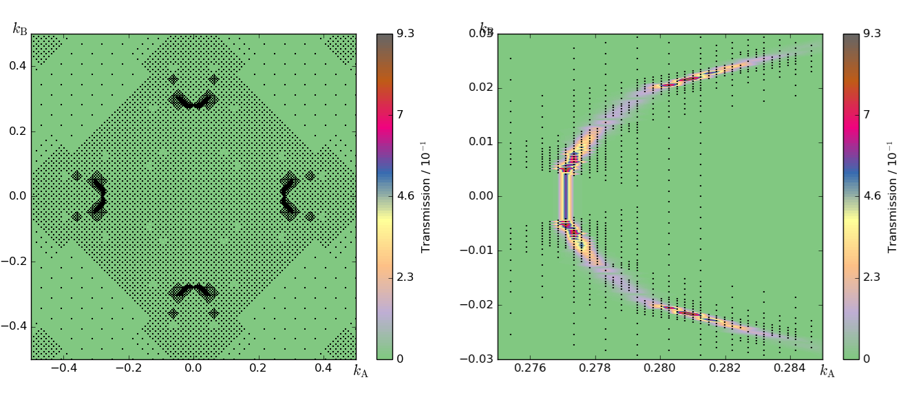
Fig. 116 Spin-down transmission spectrum evaluated using an adaptive grid using a relative tolerance of 10-2. The black dots indicate the sampled k-points. The total k-point averaged spin-down transmission is 3.5 \(\cdot\)10-5. Left: Full BZ view. Right: Zoom-in around the right-hand transmission peak.
Restricting the grid range
The AdaptiveGrid class can also be used to resolve only a specific part of the
k-dependent transmission. The script shown below (zoom.py) gives an example
of this, where the adaptive grid is restricted to specific \(k_A,k_B\) ranges,
and thereby zooms in on specific features of the spin-up and spin-down k-dependent
transmissions, respectively. A relative tolerance of 10-3 is used to fully
resolve the transmission features.
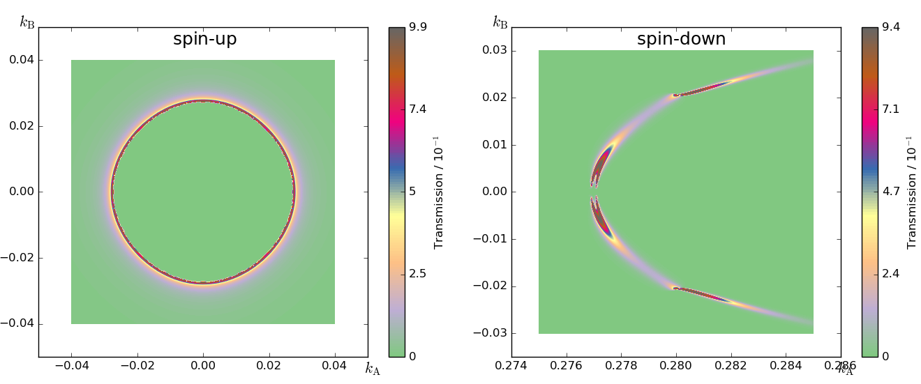
The resulting spin-up and spin-down transmissions are illustrated below. Note the different scales on the figure axes.
# -------------------------------------------------------------
# Load device configuration
# -------------------------------------------------------------
device_configuration = nlread('mgo_para.nc', DeviceConfiguration)[0]

# -------------------------------------------------------------
# Transmission Spectrum zoom #1.
# -------------------------------------------------------------
adaptive_grid = AdaptiveGrid(
    kA_range=[-0.04, 0.04],
    kB_range=[-0.04, 0.04],
    tolerance=0.001,
    error_measure=Relative)

transmission_spectrum = TransmissionSpectrum(
    configuration=device_configuration,
    energies=numpy.linspace(0,0,1)*eV,
    kpoints=adaptive_grid,
    )
nlsave('zoom.nc', transmission_spectrum)

# -------------------------------------------------------------
# Transmission Spectrum zoom #2.
# -------------------------------------------------------------
adaptive_grid = AdaptiveGrid(
    kA_range=[0.275, 0.285],
    kB_range=[-0.03, 0.03],
    tolerance=0.001,
    error_measure=Relative)

transmission_spectrum = TransmissionSpectrum(
    configuration=device_configuration,
    energies=numpy.linspace(0,0,1)*eV,
    kpoints=adaptive_grid,
    )
nlsave('zoom.nc', transmission_spectrum)
Warning
The total (k-point averaged) transmission is most likely not correct if you choose to sample only a specific part of the Brillouin zone. Use full-zone sampling to compute the total transmission through the device, which is also the default setting.
Spin-transfer torque
You will in this section compute the spin transfer torque (STT), which requires non-colinear spin. The tutorial Introduction to noncollinear spin gives for more information on how to perform STT calculations and non-colinear spin.
In the following, you will:
calculate the non-colinear device configuration;
calculate the Mulliken population and spin transfer torque.
Computing the non-colinear device configuration
The script mgo_nonco_dc.py calculates the non-colinear ground state of the device
configuration by using the colinear ferromagnetic calculation as starting point
and a density mixing scheme which diagonalizes the density matrix before mixing it.
Please, note that this script replaces the spin polarized exchage-correlation
(SGGA.PBE) by the non-colinear one (NCGGA.PBE).
# Read in the collinear calculation
device_configuration = nlread('mgo_para.nc', DeviceConfiguration)[0]

# Use the special noncollinear mixing scheme
iteration_control_parameters = IterationControlParameters(
    algorithm=PulayMixer(noncollinear_mixing=True)
    )
# Get the calculator
calculator = device_configuration.calculator()
new_calculator = calculator(
       exchange_correlation=NCGGA.PBE,
       iteration_control_parameters = iteration_control_parameters
       )
# Define the spin rotation
theta = 120*Degrees
left_spins = [(i, 1, 0*Degrees, 0*Degrees) for i in range(3)]
center_spins = [(i+3, 1, theta*i/5, 0*Degrees) for i in range(6)]
right_spins = [(i+9, 1, theta, 0*Degrees) for i in range(3)]
spin_list = left_spins+center_spins+right_spins
initial_spin = InitialSpin(scaled_spins=spin_list)

# Setup the initial state
device_configuration.setCalculator(
    calculator=new_calculator,
    initial_spin=initial_spin,
    initial_state=device_configuration)

# Calculate and save
device_configuration.update()
nlsave("mgo_nonco_dc.nc", device_configuration)
The spin setup corresponds to the spin polarization of the atoms in the left electrode pointing along the transport axis Z, while in the right electrode the polarization is rotated 120 degrees. In the central region, the angle is interpolated between these two values. Note that this is just the initial spin configuration – the actual spin polarization vectors will be computed selfconsistently and may therefore change (you can see the results in the next section).
Calculate the Mulliken population and spin transfer torque
Once the calculation is finished you can find the non-colinear device configuration in the LabFloor.
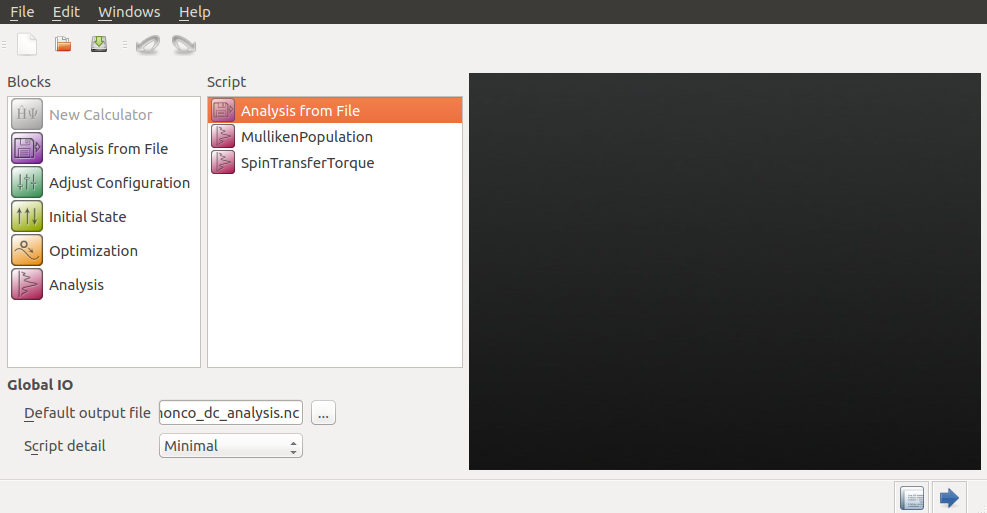
In order to calculate the Mulliken population and spin transfer torque, go to the
Script Generator and add the following blocks to the script:
 Analysis from File
- MullikenPopulation
- SpinTransferTorque
Then, change the default output file name to mgo_nonco_dc_analysis.nc.
Adjust the settings in some of the blocks:
Analysis From File:
select the
mgo_nonco_dc.ncfile.
SpinTransferTorque:
Select Left for the contributions. This way, you will calculate the left –> right linear response current.
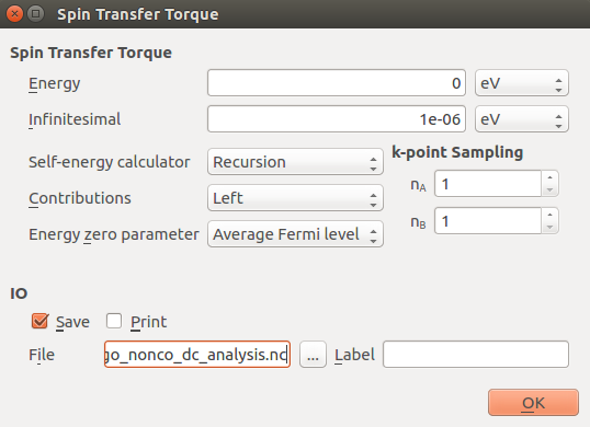
Send the script to the editor using the send to button (the icon) and replace the Monkhorst-Pack
grid with the Adaptive grid as shown below.
# Setup adaptive grid object.
adaptive_grid = AdaptiveGrid(
        kA_range=[-0.5, 0.5],
        kB_range=[-0.5, 0.5],
        tolerance=1e-2,
        error_measure=Relative,
        )
# -------------------------------------------------------------
# Spin Transfer Torque
# -------------------------------------------------------------
spin_transfer_torque = SpinTransferTorque(
    configuration=device_configuration,
    energy=0*eV,
    kpoints=adaptive_grid,
    contributions=Left,
    energy_zero_parameter=AverageFermiLevel,
    infinitesimal=1e-06*eV,
    self_energy_calculator=RecursionSelfEnergy(),
    )
nlsave('mgo_nonco_dc_analysis.nc', spin_transfer_torque)
If you wish, you can download the script here (mgo_nonco_dc_analysis.py).
The STT should be computed using a k-point sampling that is dense enough to get a well-converged value for the total torque on the right-hand side of the device. In this script we are using the adaptive grid with a relative tolerance of 10-2. The below figure shows the total spin transfer torque transfered at the right side through Fe|MgO|Fe MTJ for different relative tolerances.
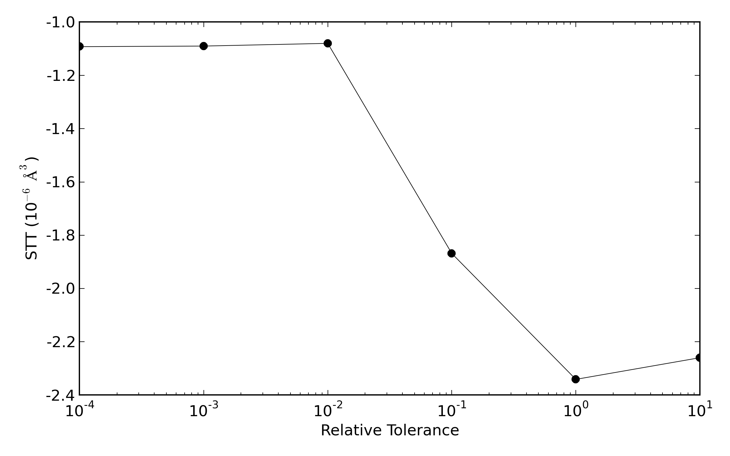
This plot shows that the use of a relative tolerance of 10-2 seems to be sufficient to obtain converged calculations of the MTJ considered in this tutorial. We have also computed the total spintransfertorque at the right side using a increasingly denser Monkhorst-Pack grid.
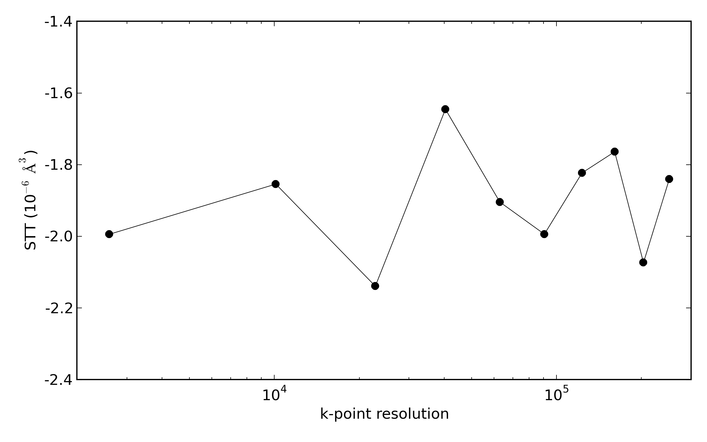
It can be seen that using a Monkhorst-Pack grid the total STT does not reach full convergece.
Analysis of the results
Once the calculation is finished, you will get the MullikenPopulation and SpinTransferTorque objects in the LabFloor. You can inspect the Mulliken charge and the component of the spin polarization vector using the text representation.
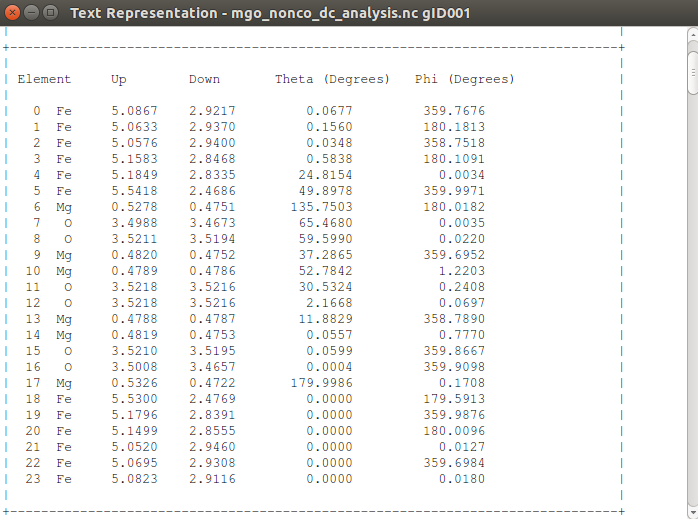
In the noncolinear calculations, the sum of the ‘up’ and ‘down’ populations corresponds
to the usual Mulliken charge (the number of electrons), and their difference –
combined with the two angles – forms the spin polarization vector. This vector can
be visualized using the  Viewer:
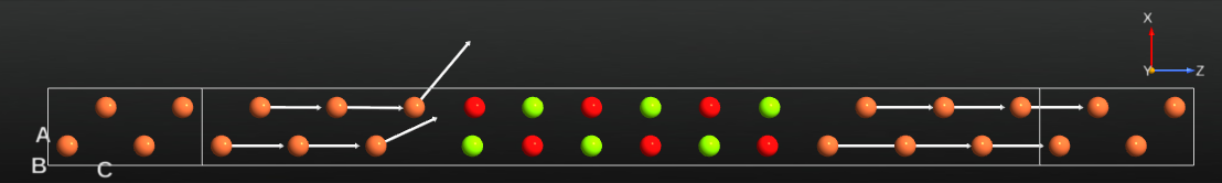
You can also plot the spatial components of the STT using the 1D Projector:

The figure below shows the MTJ configuration and the “y” component of the STT.

Relaxing the device central region
This section shows you how to create and geometry optimize the central region in the Fe|MgO|Fe junction. The tutorial Advanced device relaxation - manual workflow gives more detailed instructions for full device optimizations, including relaxed electrodes and optimum central region length. For the sake of simplicitly, we here perform force minimization for the device central region only.
Initial configuration
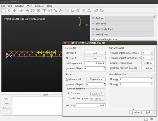
First, open the Builder. To set up the initial geometry of the
Fe|MgO|Fe device you will use the MTJ Builder plugin, which is designed
specifically for constructing this type of geometry. Locate it like this:
.
The MTJ builder can build a range of different magnetic tunnel junction geometries. For the present purpose, change the number of barrier layers to 6, and the number of surface layers to 2 on both the left and right side, but leave the other parameters as they are by default. Click the Preview button to see the geometry, then click Build to add it to the Stash.
Tip
Hover the mouse over each input field to get a description of the input parameters.
Convert the device geometry to a bulk configuration by clicking the  Bulk tool on the plugins toolbar. This simply removes the electrodes and leaves you
with the bulk central region.
Bulk tool on the plugins toolbar. This simply removes the electrodes and leaves you
with the bulk central region.
Geometry optimization
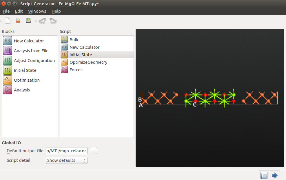
Send the device central region to the Script Generator
and add the following blocks to the script:
- New Calculator
- Initial State
 OptimizeGeometry
- Forces
Also, change the default output filename to mgo_relax.nc
The Calculator and InitialState settings should be very similar to those used in section Parallel spin:
Calculator:
Select the SGGA exchange-correlation method.
Increase the electron temperature to 1200 Kelvin.
Set the k-point grid to 7x7x2. This choice gives a reasonable k-point sampling in the x and y directions. In the z direction, you would like to model a device configuration, so the iron atoms at the edges must be bulk-like. Selecting 2 k-points in the z-direction improves the bulk like description of the Fe edge atoms.
Select the SingleZetaPolarized basis set for iron.
Initial State:
Choose User spin for as the type of initial state.
Set the relative spins on O and Mg atoms to 0.
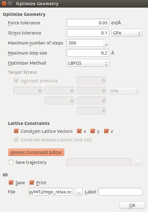
Next, open the Optimization block to specify that
the first and last four atoms in the central region (the atoms in the electrode extensions)
should be kept fixed during the relaxation. This is very important – if any of these atoms
move you no longer have a periodic structure at the edges of the central cell, which is
required for generating and attaching device electrodes later on.
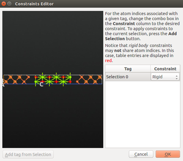
Click Add Constraints to open the Constraints Editor. Then do the following:
Select the atoms indicated in the image below by holding down the Ctrl key and drawing a rectangle around them. Then click Add tag from Selection to assign the tag “Selection 0” to those atoms. Change the constraint type to “Rigid” for this tag group.
Do the same for the right-hand electrode extension atoms, but leave the constraint type as “Fixed”.
Save the script as mgo_relax.py and run it using the
Job Manager or from the command line:
atkpython mgo_relax.py > mgo_relax.log
If needed, you can also download the script here: mgo_relax.py. This calculation will
take a 1-2 hours on a standard PC, but may finish in 20 minutes if distributed over
4 parallel MPI processes.
Inspecting the results
Locate the calculation data items on the LabFloor. Select the Forces item (gID002), and click the Text Representation plugin. You will now see a report of the final forces on all atoms.
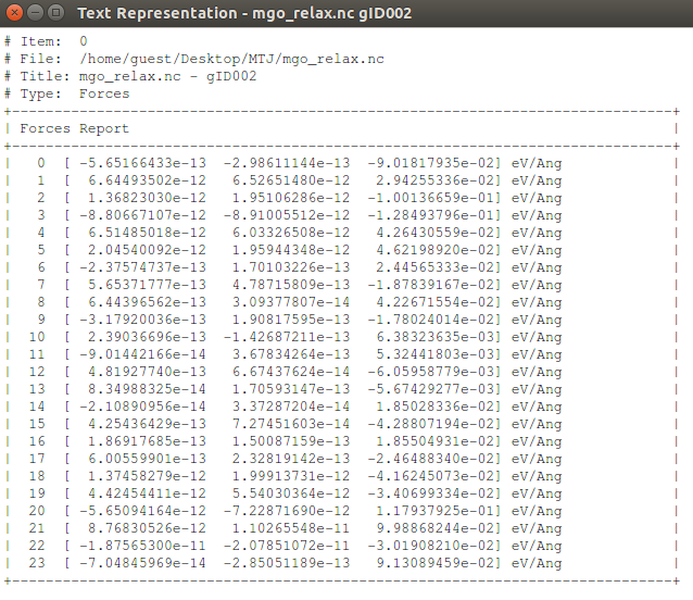
Note that all forces in the x-y direction are for all practical purposes zero. For the atoms which have been relaxed, the forces are less than the optimization criterion of 0.05 eV/Ang. For the electrode extension atoms, the forces are slightly larger. Moreover, the force vectors point out of the cell, indicating that the cell is under compressive strain. Adding more surface layers to increase the cell length in the z-direction would lower the strain, but would have very little effect on results in the present case.
You can now use the optimized device central region for calculations of transport properties of the device, c.f. section Getting started.