Moment Tensor Potential (MTP) Training for Crystal and Amorphous Structures
Moment Tensor Potential (MTP) Training for Crystal and Amorphous Structures
Version: Y-2026.03
In this introductory tutorial, you will learn how to use QuantumATK to
Set-up a workflow for training a machine-learned force field (ML FF),
MTP, for crystal and amorphous TiSi and TiSi2 structures,
which can be used for molecular dynamics (MD), geometry optimization, and
other force-field-based simulations.
Analyze the MTP training results.
Validate the quality of the trained MTP.
Unlike many empirical potentials with physical functional forms, ML FFs
such as MTPs are not highly transferable and must be trained with the target
application in mind. For example, an MTP trained for bulk structures will not
describe accurately free surfaces or nanoparticles of that material without
the addition of such structures to the training set.
However, the outlined training protocol can be easily adapted or extended to
train an accurate MTP for different geometries, stoichiometries, element
composition and other materials by explicitly including relevant training data
for such structures.
Note
Framework Update: This tutorial has been revised to use the new ML FF
training framework, which separates the workflow into dedicated classes:
The previous MomentTensorPotentialTraining class is deprecated but
existing workflows will continue to function.
Parts of this tutorial have been re-run using the new framework, while some
results are carried over from the previous version. The outcomes should be
comparable, but minor differences may occur.
ML FFs are trained to predict ab initio, i.e., DFT, potential energy
surfaces (PES) and vastly improve the accuracy of classical dynamics
simulations while keeping the computational cost at the level of empirical
force fields. To train a ML FF, one first needs to calculate training data
(energy, forces, stress) for generated training configurations (typically, of
relatively small sizes) with the reference DFT calculator and then fit an MTP
to that DFT training data. Simulations with trained ML FFs can reach the high
accuracy, long simulation times and large system sizes that capture the
complexity of realistic systems, e.g., amorphous and alloy materials, and
processes, e.g., diffusion, crystallization or deposition.
QuantumATK implemented Moment Tensor Potentials (MTPs)
[1] as they provide high performance for a given
accuracy when compared to other ML FFs models in the literature
[2]. MTP advantages include:
Very fast and supports large scale simulations.
Allows training to multi-element-materials.
Systematically improvable.
Tip
Since the MTP is trained to match the DFT reference calculator results,
the accuracy of the final MTP is tied to this choice. Thus, it is
important to choose the reference calculator that gives a good
description of the system and application you want to study.
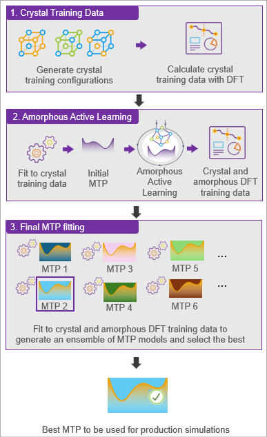
MTP training for crystal and amorphous structures in QuantumATK is
structured into three stages:
Crystal Training Data - generates crystal training configurations
with random displacements and calculates training data (energy, forces,
stress) with the reference calculator DFT. Crystal training data forms
the bulk of the training set, giving a fundamental description of the
material in question. It will also be used to fit an initial MTP in the
2nd MTP training stage.
Amorphous Active Learning - fits an initial MTP to the crystal
training data, which is then used to run iterative Active learning
geometry optimization and MD simulations to identify relevant
configurations which are not represented in the initial training set.
This workflow actively adds extrapolating amorphous configurations, incl.
DFT data, to the training data set. The combined amorphous + crystal
training data is then used in the 3rd stage to fit an ensemble
of MTP models.
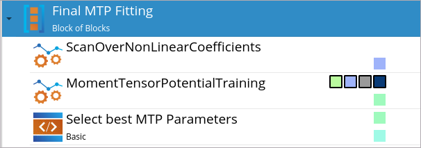
Final MTP Fitting - generates an ensemble of MTP models with
different initial non-linear coefficients and selects the best fitted MTP
that gives lowest and comparable training and testing errors with respect
to the reference DFT method.
The chosen MTP can then be used in production simulations, such as MD,
geometry optimization, and other force-field-based simulations.
Download the ready-to-use MTP training workflow
c-am-TiSi-MTP-training.hdf5 and open it in the
Workflow Builder.
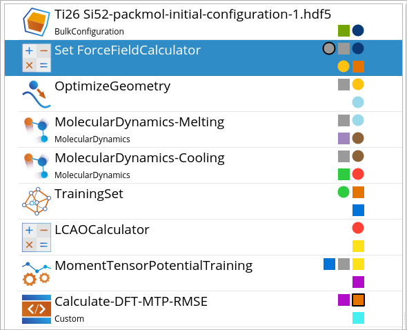
The workflow consists of three aforementioned stages (each contained in a
so-called Blocks of Blocks) and is applicable to any crystal and
amorphous material:
Crystal Training Data
Amorphous Active Learning
Final MTP Fitting
The LCAOCalculator block placed above
the three Blocks of Blocks is used for defining a reference DFT-LCAO
calculator (using the PBE xc-functional) that is used to calculate
training data (energy, forces and stress) throughout the MTP training
simulations.
Under the Main tab, the k-point density is increased from the
default medium to high, i.e., from 4Å x 4Å x 4Å to
7Å x 7Å x 7Å, to reduce the impact of sampling discontinuities when
slightly changing the cell size during random displacements of the
structure.
Under the Iteration Control tab, the SCF Tolerance is decreased from
the default 1e-04 to 5e-05 to reduce the noise in energy, forces,
stress, and the Max steps for SCF is increased from default 100 to
200 so that SCF also converges even if the configuration needs more
steps due to the tighter tolerance.
Under the Algorithm tab ‣ Parameters, the default Optimize
diagonalization for memory is switched to Optimize diagonalization for
speed.
We will now go through the three stages step-by-step, explain the settings,
and provide tips and recommendations.
We will begin with the 1st stage of the MTP training workflow -
Crystal Training Data. This includes generation of crystal training
configurations, i.e., repeated and randomly displaced crystal structures of
different phases of titanium silicide using the
crystalTrainingRandomDisplacements protocol, and calculation of
training data with DFT for these displaced configurations.
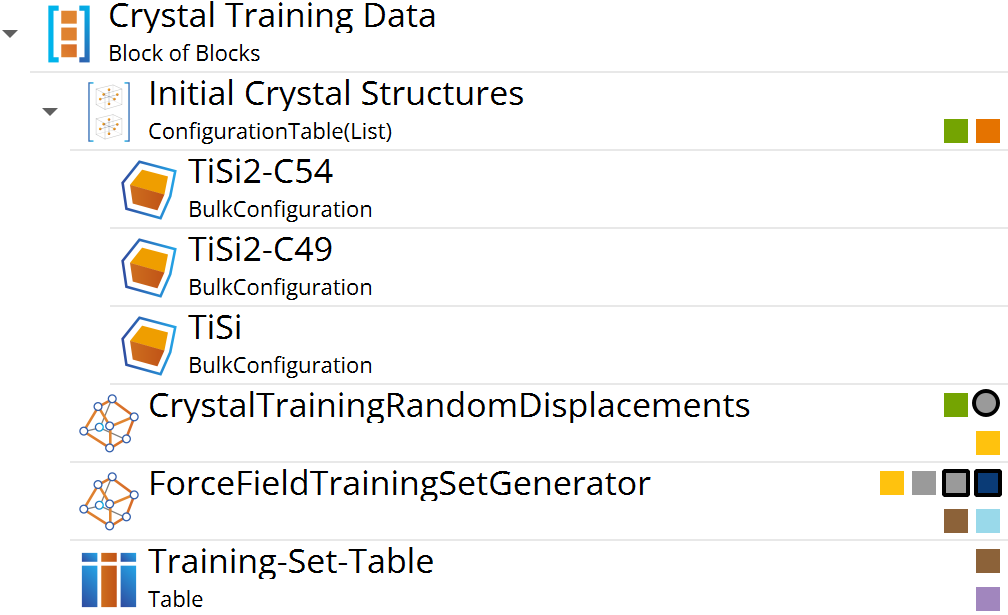
The Initial Crystal StructuresConfigurationTable(List) block
contains three crystal structures of titanium silicide, with two different
stoichiometries, which we will include in the MTP training: TiSi,
TiSi2-C54 and TiSi2-C49. These structures will be used for
generating randomly displaced structures - the training configurations.
Note
The required input for the Initial Crystal Structures depends on the
application of the final trained MTP. If you intend to use the trained MTP
for simulating other stoichiometries and crystal phases than TiSi,
TiSi2-C54 and TiSi2-C49, then you should include structures
with these “other” stoichiometries and crystal phases as well, to ensure
accurate simulations for those materials.
Tip
Crystal structures can be imported from the NanoLab’s Internal Database
in the Builder or from the Materials Project
database in the Databases.
It is recommended to optimize the geometry of crystal structures with
the reference (DFT) calculator before using them for the MTP training.
The CrystalTrainingRandomDisplacements block sets parameters for
randomly displacing configurations around the equilibrium of the provided
crystal structures of titanium silicide.
System sizes: Define the target sizes for the supercells in which the
atoms will be displaced. It is recommended to use at least 2 different
sizes (in this case, 20 and 50), so that the MTP model can better
learn the system-size dependence of the total energy.
Target sample size: Set the minimum for how many displaced
configurations should be generated. Note that depending on various input
choices, the final number of training configurations can be significantly
higher. Here, we choose 200 (default).
Base / max atomic rattling amplitudes: Define by what magnitude the
atoms are displaced. Should be chosen so most displaced configurations
have max. atomic forces below 5 eV / Ang, and that the max. atomic forces
peaks are between 20 – 40 eV / Ang. The default values (0.15 Å/ 0.4 Å)
work well for most materials, but for pure metals larger values can be
chosen (e.g. 0.25 Å / 0.55 Å).
Include strain: Should be enabled (by default), unless not needed for a
specific application.
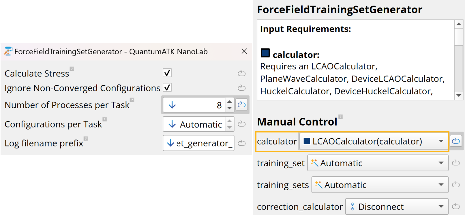
The ForceFieldTrainingSetGenerator block sets parameters for
calculating DFT training data (energy, forces, stress) for the randomly
displaced configurations.
This class is specifically designed for generating and calculating
training data.
Number of processes per task: Specify how many MPI processes should be
used for each DFT calculation (default - all available processes).
Since the DFT calculations are mostly independent from each other,
multiple DFT calculations can be done at the same time. For example, when
submitting a calculation on 40 MPI processes, number of processes per
task could be 8, thus resulting in 5 DFT calculations running at the
same time. This can speed up the entire calculation, but will use more
memory.
Calculate stress: Should be enabled (by default) to include stress in
the training data.
LCAOCalculator and ForceFieldTrainingSetGenerator blocks must be
connected, so that the defined LCAOCalculator is used to calculate
training data.
The generated training data with DFT is exported as a TrainingSet
object, which can be retrieved from the ForceFieldTrainingSetGenerator
using the generatedTrainingSet() method.
Note
In case of training an MTP model for the use of crystal applications only,
one could take the TrainingSet generated above and directly move to the
3rd stage - Final MTP Fitting. The resulting MTP would be able
to describe the trained crystal phases up to medium temperatures (i.e.,
well below the melting point where the crystal is still stable). Crystal
properties, such as lattice constants, elastic moduli, or phonons, are
typically described very well using this training data.
In the 1st stage of the MTP training we generated crystal training
data for the initial MTP fitting. In the 2nd stage, Amorphous
Active Learning, we will include training data for amorphous configurations.
Here, it is not so straightforward to identify all relevant amorphous
configurations beforehand, thus we will employ the
ActiveLearningSimulation approach for on-the-fly improvement of
training dataset by actively adding extrapolating amorphous training
configurations from dynamic simulations, such as geometry optimization and
melt-quench MD.
Note
Active learning is a strategy for iteratively finding and selecting new
atomic configurations for which the MTP has the highest uncertainty,
i.e., highest prediction errors (so-called extrapolating
configurations). These configurations are most likely to improve the
MTP’s overall accuracy and robustness when added to the training data
set, especially for configuration outside he original training data
domain. Since Active learning targets specific configuration spaces
instead of randomly sampling configurations, it reduces the need for
expensive DFT training data calculations, which leads to efficient and
fast training.
It is recommended to include Active learning when training an MTP for
amorphous systems, interfaces, surface processes, and systems at high
temperatures.
In addition to geometry optimization and MD, methods such as NEB, AKMC
and TFMC can also detect extrapolating configurations and add them to the
training data set.
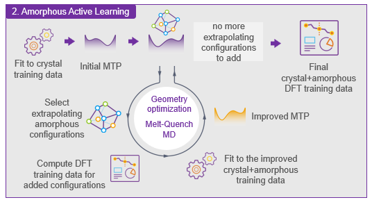
During Amorphous Active learning, first, one fits an initial MTP to the
crystal training data and then iteratively repeats the flow below until there
are no more extrapolating configurations to add, as also shown in the figure
below:
Perform geometry optimization and MD melt-quench (melting/cooling)
simulations with the current MTP to find additional extrapolating
amorphous training configurations.
Calculate DFT training data for these added training configurations.
Fit a preliminary MTP to the improved training data.
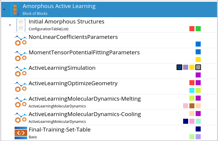
The actual workflow for the Amorphous Active Learning stage in the
Workflow Builder looks like this:
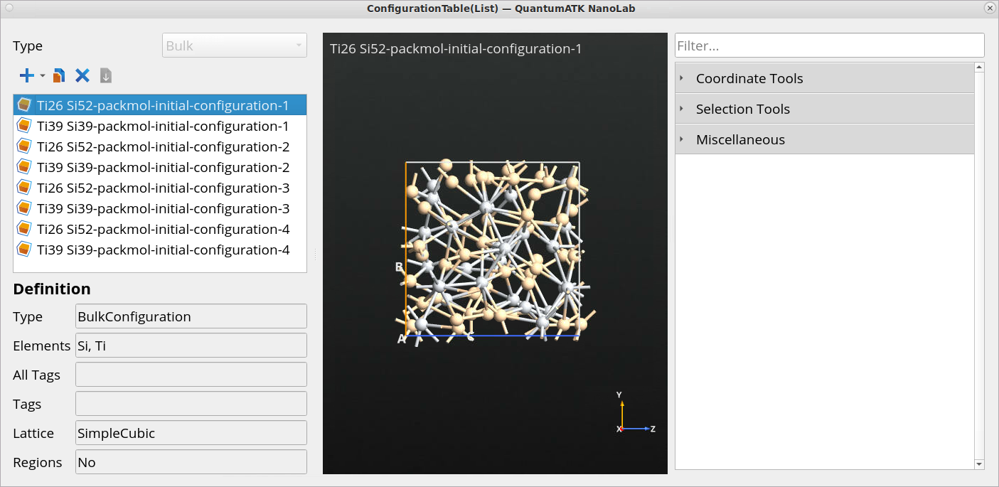
The Initial Amorphous StructuresConfigurationTable(List) block
contains initial amorphous structures of titanium silicide, where each of
them will be used as a starting point for Active learning
GeometryOptimization and ActiveLearningMolecularDynamics simulations.
Since we have eight initial amorphous Ti39Si39 and
Ti26Si52 structures, QuantumATK will perform eight
Active learning geometry optimization and eight subsequent Active learning
MD melt-quench simulations.
Tip
Initial amorphous configurations can be generated using Packmol in the
Builder as showcased in the tutorial
Molecular Dynamics Simulations for Generating Amorphous Structures or can be generated on-the-fly using the
AmorphousPrebuilder block in the Workflow
Builder.
Now let’s set up the generation of MTP fitting parameters that will be fitted
to the training set data by minimizing the error (energy, forces and stresses)
with respect to the reference DFT calculator.
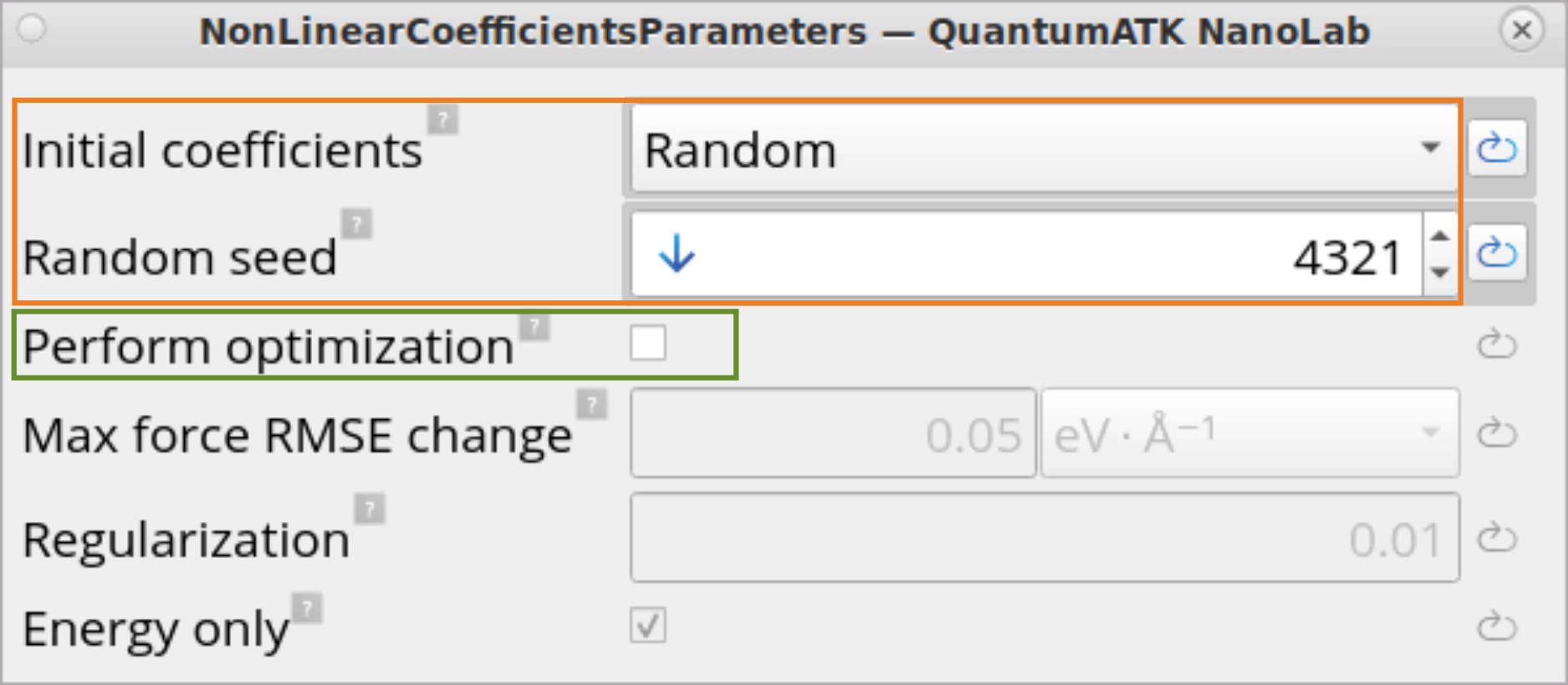
The NonLinearCoefficientsParameters block contains settings for
randomly generating non-linear coefficients for the radial functions for
each element pair (see NonLinearCoefficientsParameters for more
info), that will be used in the next step - calculation of MTP fitting
parameters (see MomentTensorPotentialFittingParameters for more
info).
Initial coefficients: Set to Random to use random values for initial
non-linear coefficients.
Random seed: Set to an arbitrary number, but use the same number for
different Active learning runs. This way consistent results are achieved
between different Active learning runs.
Perform optimization: Recommended to keep it unchecked in the
Amorphous Active Learning stage as non-linear MTP training (optimizing
non-linear coefficients) usually does not give much improvement in
accuracy and it will increase the calculation time.
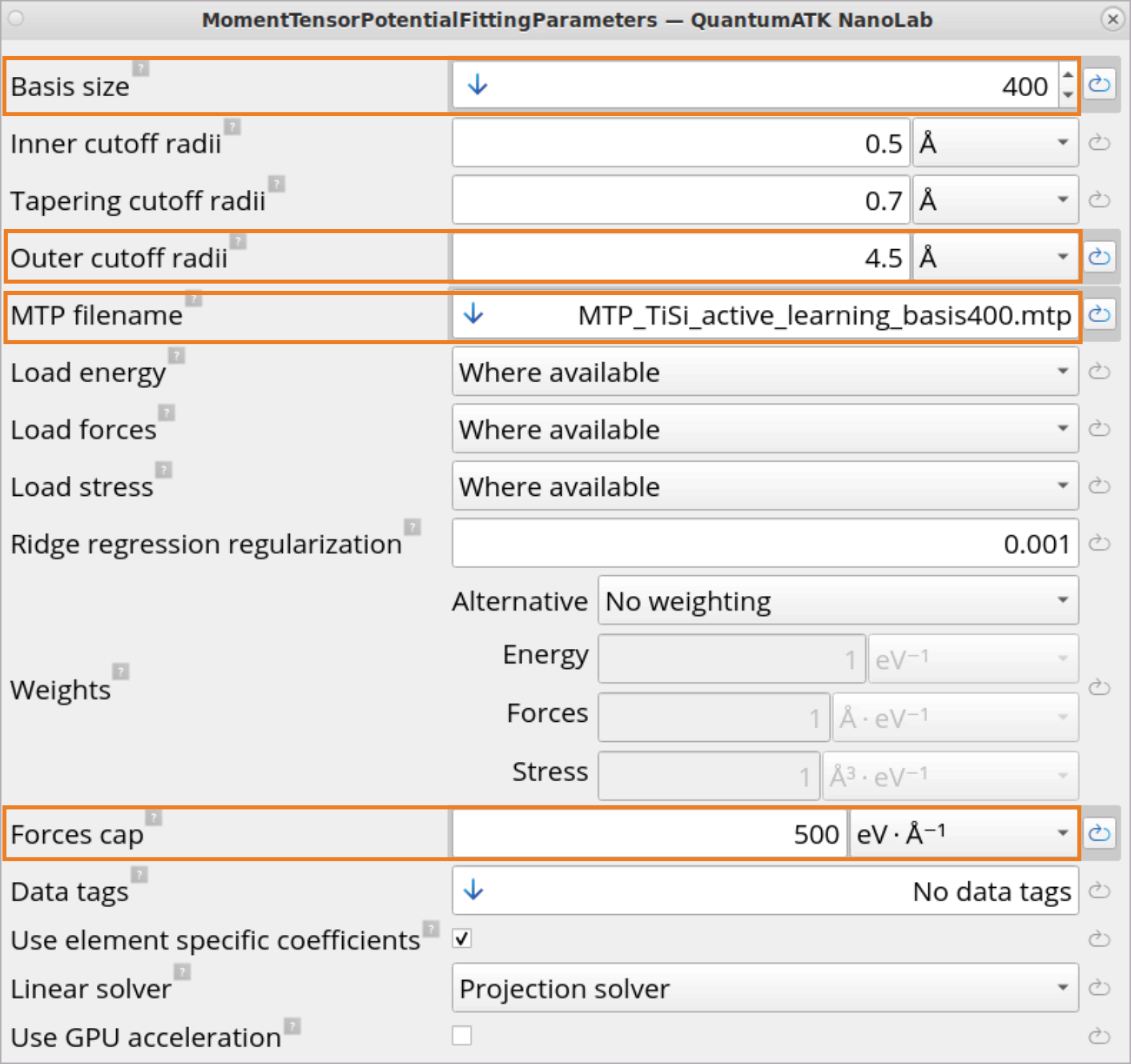
The MomentTensorPotentialFittingParameters block contains settings for
MTP fitting using the non-linear coefficients generated in the previous
step.
Basis size: Use 400 basis functions in this example. Generally, it is
recommended to use either Predefined Basis Small (default), or between
300 – 800 basis functions. More basis functions usually provide a better
accuracy (lower training error), but the simulation can become less
stable, especially in out-of-equilibrium situations, e.g., at high
temperatures or energies.
Outer cutoff radii: Set to 4.5 Ang in this example. This value
specifies the range of the atomic environments. Typically values between
4-5 Ang are recommended. Similar to basis size, larger values can
increase accuracy, whereas smaller values can provide more stability.
MTP filename: One should always specify a filename with .mtp
extension. This is where the trained MTP parameters are stored.
Forces cap: Specify this value in order to exclude configurations with
very large forces, i.e., above the Force cap, from the training. For
Active learning it is always recommended to set this to a relatively large
value, e.g. 500 eV / Ang, to include closer atom distances with larger
forces in order to make sure the repulsive behavior is predicted correctly
in such situations. Increasing the Forces cap (within some limit) makes
the simulation more stable, but less accurate. Thus, while setting the
Forces cap, one needs to balance between simulation stability and
accuracy.
Note
Within the MTP framework, the total energy of a configuration is computed as
the sum of energy contributions from atomic environments. Atomic
environments are defined as the representation of the immediate chemical
environment of each atom in the system within a cutoff radius. Moment
tensors include the radial, angular, and many-body distribution of atoms
within a cutoff sphere. Their contractions into scalar basis functions
provide an invariant representation of atomic environments (‘structure’) as
input for MTP training [1].
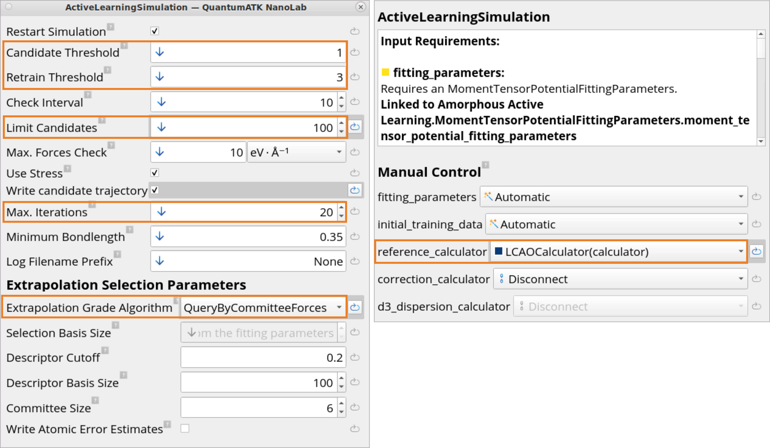
Now let’s set up Active learning simulation parameters.
The ActiveLearningSimulation block contains settings for running Active
learning simulations. MTP fitting parameters from the previous step and the
initial training data from the crystal training are used as an input.
Candidate/ Retrain Threshold: These are numerical measures governing how
much configurations can differ from the training set before they are
considered to be extrapolating. If the current configuration has an
extrapolation grade higher than the candidate threshold (default 1), it
will be kept as a possible candidate to be included in the next training.
If the value is larger than the retrain threshold (default 3), the
current simulation will be stopped, extrapolating configurations will be
added to the training data set, and then Active learning will be
re-started now using an improved MTP fitted to the extended training data
set.
Limit candidates: Set to 100. Limit the number of recorded candidates
for each simulation. This can be beneficial in case the simulation moves
between candidate and retrain threshold for a long period and many
candidates are registered. In that case the candidates are typically very
correlated and not all of them are needed. The limited candidates are then
taken from the raw list of candidates at a regular interval, before a
structural filter extracts the most different configurations and adds them
to the training set.
Max. Iterations: The maximum number of re-training iterations, i.e., how
many times the simulation will start again with a new MTP. Stick to the
default value. It can be increased if more iterations are expected.
Extrapolation grade algorithm: Select which algorithm is used to
calculate the extrapolation grade. Unless there is only a single element
in the simulation, we always recommend to set this to
QueryByCommitteeForces.
LCAOCalculator and ActiveLearningSimulation blocks must be connected,
so that the defined LCAOCalculator is used to calculate training data
during Active learning.
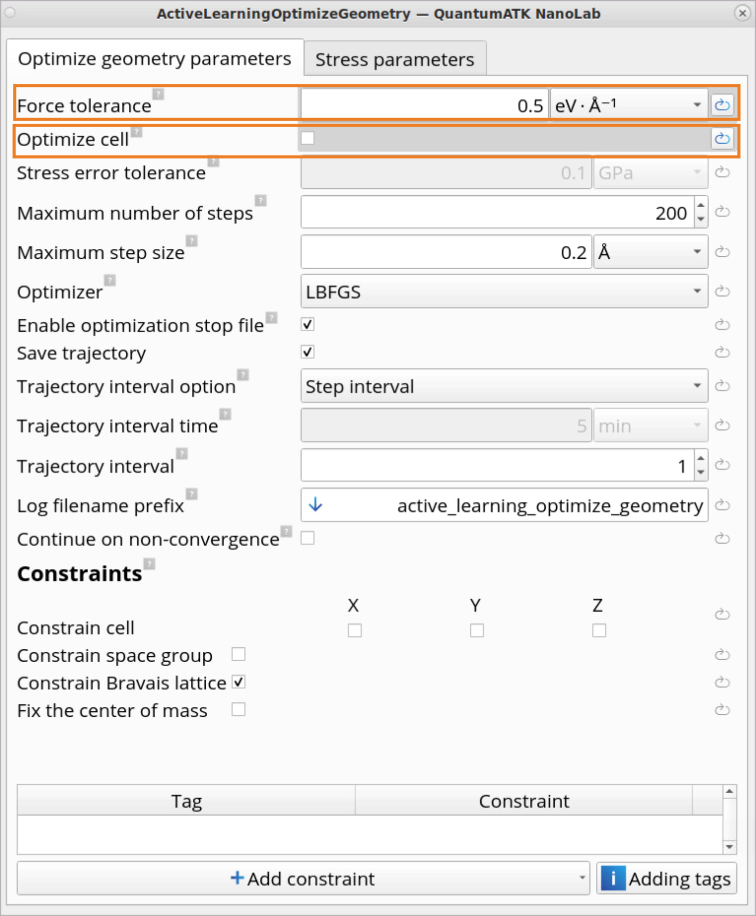
The ActiveLearningOptimizeGeometry block contains settings for
performing Active learning geometry optimization. All initial amorphous
configurations from the Initial Amorphous StructuresConfigurationTable(List) block will be used as a starting point for the
ActiveLearningOptimizeGeometry. The optimizations will be run
independently and in parallel (as much as the parallel settings allow that,
otherwise sequentially). The DFT calculations and training are done
collectively, using the combined extrapolating candidate configurations
selected from all optimizations.
Force tolerance: set a bit higher than the default, i.e., to
0.5 eV / Ang, as this part should primarily do a quick pre-optimization
to avoid large forces in the active learning MD part.
Optimize cell: this is disabled to make the optimization more robust.
The combined crystal training + amorphous geometry optimization training data
is used to train an improved MTP, which is then used for subsequent Active
learning melt-quench MD simulations.
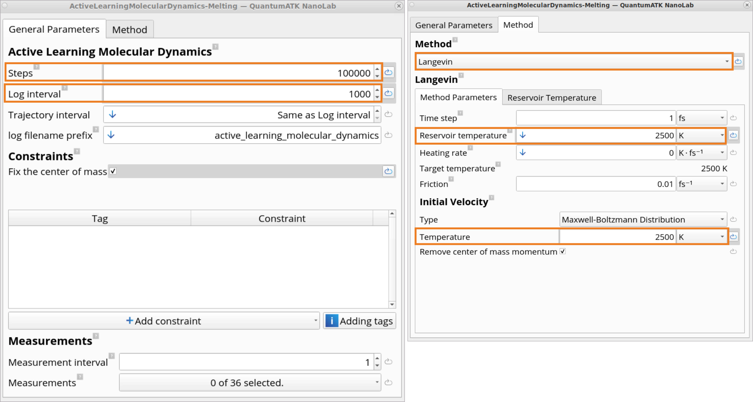
The ActiveLearningMolecularDynamics-Melting block contains settings for
performing Active learning MD melting simulations. Here, we want to run MD
at relatively high temperatures to melt the disordered configurations and
sample many different relevant atomic environments.
Steps: set to 100 000 MD steps and set Log interval to 1000 MD
steps.
Method: set to Langevin.
Reservoir temperature and Temperature of initial velocities is set to
2500 K to melt the disordered configurations.
Tip
One can also use a different thermostat type than Langevin, however, to
ensure the simulation is relatively robust one should pick a robust
thermostat, like Berendsen or Bussi-Donadio-Parrinello. At such high
temperatures, it is recommended to run NVT simulations, whereas NPT
simulations should primarily be run at lower temperatures.
Note
The chosen Active learning MD temperature should reflect a physical
process (e.g., chemical reactions, phase transitions, or material
properties) that occur within a specific temperature range and that you
want to simulate in production simulations with a trained MTP.
The temperature should not be too low as it would miss configurations
relevant at high temperatures (e.g., disordered amorphous structures).
The temperature should also not be too unphysically high, as in that case
the system may visit configurations that are physically unrealistic, or
not representative of the system’s true equilibrium state. In addition,
due to too high temperature, the system may also fail to properly sample
the configuration space by jumping over energy barriers rather than
exploring the free energy surface in a smooth, gradual manner.
To sum it up, too low or too high temperature could result in the reduced
accuracy of Active learning and thus the trained MTP.
The combined crystal training + amorphous geometry optimization + amorphous MD
melting training data is used to train a further improved MTP, which is then
used in subsequent Active learning MD cooling simulations.
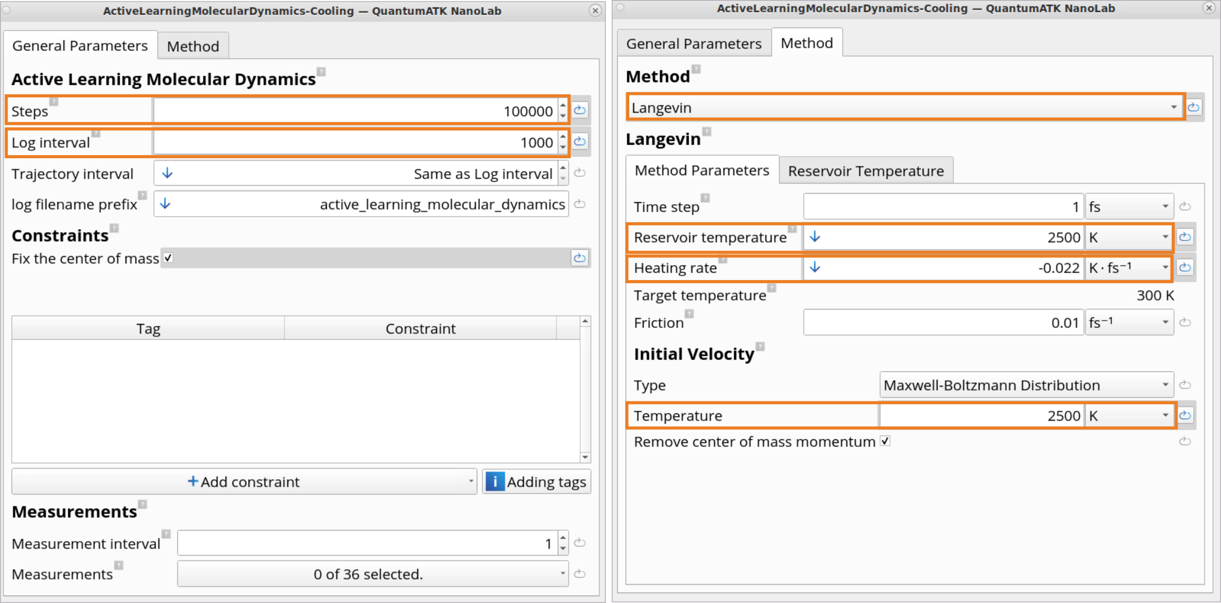
The ActiveLearningMolecularDynamics-Cooling block contains settings for
performing Active learning MD cooling simulations - to simulate cooling the
liquid configuration to room temperature.
Steps: set to 100 000 MD steps and set Log interval to 1000 MD
steps.
Method: set to Langevin.
Reservoir temperature and Temperature of initial velocities is set to
2500 K, but now we specify a negative heating rate of
-2200/100 000 K/fs to decrease the temperature from 2500 K to 300 K
during the 100 ps of MD.
The Final-Training-Set-Table block picks up the Training-Set-Table
containing the combined data from crystal displacements and Active learning
and exposes it under a more obvious name, so that it can easily be used in
the following Final training stage.
In the 2ndAmorphous Active Learning stage we did preliminary MTP
fittings to generate amorphous training data for titanium silicide on-the-fly.
For this, we used only one set of initial non-linear MTP coefficients. In the
3rd stage, Final MTP Fitting, we will fit an ensemble of MTP
models to the crystal+amorphous training data and select the best fitted MTP.
We will scan over 30 different initial guesses of non-linear MTP coefficients
to generate different fitted MTPs based on these initial guesses. We then
select the one which gives the lowest, and comparable, training and testing
errors with respect to DFT. This can then be used in production simulations.
The actual workflow for the Final MTP Fitting stage in the
Workflow Builder looks like this:
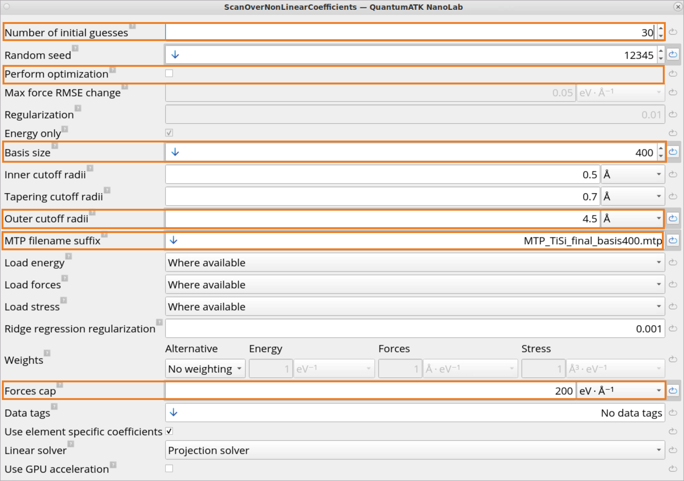
Number of initial guesses: Defines how many different initial values
should be considered. The default value of 30 is usually sufficient.
Increasing the number means a better chance of finding the best possible
MTP at a cost of an approximately a linear increase in the calculation
time. This is mainly recommended for complex training data with many
elements.
Basis size: Use 400 basis functions for this example (same as in
active learning). Generally, it is recommended to use either
Predefined-Small, or between 300 – 800 basis functions. More basis
functions usually provide a better accuracy (lower training error), but
the simulation can become less stable, especially in out-of-equilibrium
situations, e.g., at high temperatures or energies. For calculations which
require a high accuracy, but not stable MD, it can be meaningful to
increase the number of basis functions beyond this range. In rare cases,
mainly for calculations which require a very high accuracy, such as
precise phonon calculations or defect energies, it can be meaningful to
increase the number of basis functions to as much as 5000.
Cutoff radii: Inner and tapering cutoff radii rarely need to be changed
from their defaults. The outer cutoff radius should be set to the same as
in Active learning (4.5 Å), as the extrapolation behavior will depend
on this choice.
MTP filename suffix: Specify the filename, where the MTP parameters are
written to. The different fits will create files such as
0_mtp_filename_suffix.mtp, 1_mtp_filename_suffix.mtp, etc.
Forces cap: Specify this value in order to exclude configurations with
large forces. In this stage it does not have to be as large as for Active
learning, we recommend 100 -200 eV / Ang for most cases, unless the
application explicitly requires to be able to deal with very large forces
(e.g. impact of high-energy ions). We choose 200 here, so that some
large forces are included to train the MTP to be able to deal with close
atoms, that might occur during the melting MD simulations.
Perform optimization: Run a separate, local optimization of the
non-linear coefficients. This takes much longer, and in most cases it
gives very little improvement in accuracy, therefore it is recommended to
have it disabled (default).
Committee size: Number of committee models to train and store using the
same data and hyperparameters for the MTP MD uncertainty predictions. This
can be set to a small number (we recommend 6). The committee model can
then be used in MD simulations to obtain an estimate of the energy and
forces error during the production simulations with a trained MTP, using
the MolecularDynamicsErrorPredictionHook.
Note
Training committee models is not strictly necessary for basic MTP training
and validation. It adds complexity to the workflow and makes the log files
more verbose with outputs from multiple committee models. However, it is
included in this tutorial for completeness, as committee models can be useful
for uncertainty quantification in production simulations. For simpler
workflows, you may omit committee training entirely.
Tip
ScanningOverNonLinearCoefficients is kind of a non-linear MTP
optimization, but a crude one in that one just tests many initial guesses
and then picks the best one (without the explicit local optimization of
non-linear coefficients). For systems that do not have too many elements
it works well.
If the number of elements becomes larger (5+ different elements), it can
be beneficial to use the particle-swarm-optimization (PSO) method
ParticleSwarmOptimizationParameters to optimize the non-linear
parameters instead of scanning over different initial guesses. This will
take longer, but provides a more systematic optimization and often results
in a better accuracy for complex systems. Since we only have 2 elements in
the system we use here, we will not use PSO in this tutorial.
The MultipleMachineLearnedForceFieldTrainers block contains settings
for training and analyzing multiple MTP models based on 30 different sets
of MTP fitting parameters. See
MultipleMachineLearnedForceFieldTrainers to learn more.
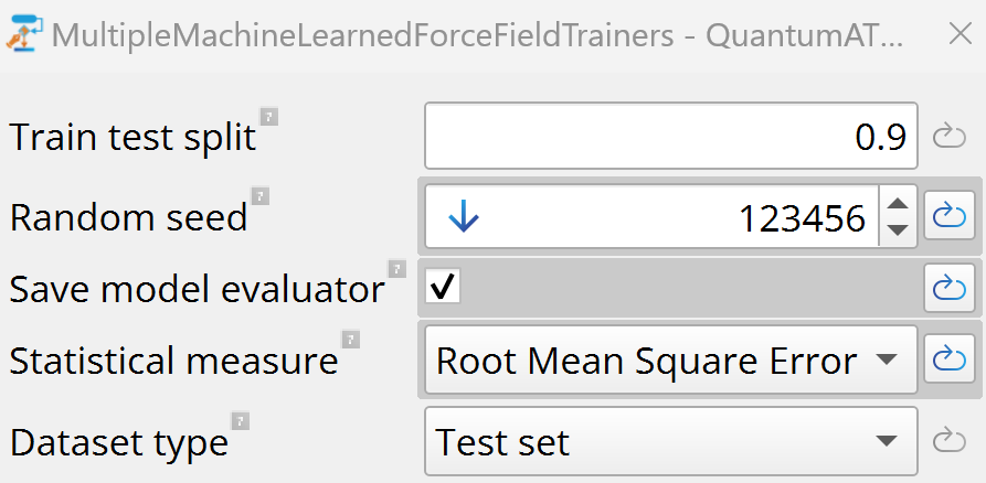
Train test split: Set it to 0.9 to use 90 % of the calculated
reference data for training and 10 % for testing. The split is done
randomly. Specify an arbitrary number for the random seed to make it
deterministic and reproducible, e.g., if one wants to change other
hyperparameters like a cutoff radii or a basis size later and compare the
results.
Statistical measure: The metric used to compare and rank models. Set it
to RMSE. Other options include R2Score and MAE.
Dataset type: Specifies whether to use training or test dataset
statistics for model comparison (default is Test set).
Ensure that the MultipleMachineLearnedForceFieldTrainers block is linked
to the Final-Training-Set-Table created in the end of the Amorphous
Active Learning section, ScanOverNonLinearCoefficients fitting
parameters list, and LCAOCalculator blocks.
Note
We use random numbers to initialize the coefficients for the MTP training,
randomly displacing crystal configurations and training-test set splitting.
Therefore, reproducibility of the results to the numerical accuracy is
only ensured if you use the same Random seed while re-running the MTP
training simulation.
Many different sets of MTP parameters could result in similar results as
there could be many degenerate minima in the hyper-parameter surface. Thus
it is not a cause for concern if you get different sets of MTP fitting
parameters with similar accuracy.
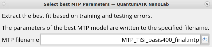
The Select best MTP Parameters block is for selecting the best fitted
MTP from 30 generated MTPs based on training and testing errors.
The getBestModel() method can be used to retrieve the best performing
model based on the specified statistical measure and dataset type.
The best model’s calculator can be retrieved using
bestFittedCalculator() method.
MTP filename: The parameters for the best fit are written to this file.
It should have the extension .mtp. This mtp file is what you will
use for setting up production simulations with the trained MTP.
The MTP training set-up is now finished and you are ready to submit this job.
Change the Workflow name and Filename as needed (e.g.,
c-am-TiSi-MTP-training-results.hdf5).
Click on the Send content to other tools button
and choose Jobs as a script to send the workflow to the
Jobs tool to submit this job on a local machine or a
remote cluster. It is recommended to use MPI parallelization for MTP
training simulations, as both training data calculations with DFT and MTP
fitting benefit from MPI parallelization.
This also generates a Python script
c-am-TiSi-MTP-training-results.py, based on this workflow. It can
be opened and edited with the Editor tool and then
sent to the Jobs tool, if you need to make manual
changes.
Estimate of the MTP training run-time: in our test it took 5 hours on the
40-core machine.
c-am-TiSi-MTP-training-results.log: The main .log file
contains a lot of information about the progress of the overall simulation,
while the DFT training data, Active learning geometry optimization and MD
log outputs are written to separate files. The most important parts of the
c-am-TiSi-MTP-training-results.log file are:
Completion of Active learning geometry optimization and melt-quench MD
simulations, reporting the number of added extrapolating amorphous
training configurations. For titanium silicide, 17, 0 and 0 extrapolating
amorphous configurations were added during Active learning geometry
optimization, MD melting and cooling phases, respectively.
Machine Learning Model Evaluation Report is shown for each of the 30
candidate fits trained by the
MultipleMachineLearnedForceFieldTrainers, where each corresponds
to a different initial guess for the non-linear coefficients. This shows
the Root Mean Square Error (RMSE), Mean Absolute Error (MAE) and
r2 values for energy, forces and stress for both training and
testing datasets, with respect to the reference DFT calculator. It also
shows the size of the training set (212 configurations ∼90% of all
training configurations) and testing set (24 configurations ∼10% of all
training configurations).
Machine Learned Model Collection Summary is reported in the end of the
.log. It shows a collective overview of all the errors using the
MachineLearnedModelCollection - here using the RMSE rankings. In
this case, QuantumATK reports the MTP fit number 11 to be the best, as
this has the lowest average RMSE value across energy, forces and stress
for the test set. The best fitted MTP is written to
MTP_TiSi_basis400_final.mtp, which can then be used for validation
and production simulations. All the 30 fitted MTPs are written to files
0,...,29_MTP_TiSi_final_basis400.mtp.
r2 values, coefficient of determination, indicate how good the MTP
is at predicting the trained properties in the dataset, with values closer
to 1 being better. Looking at the individual MTP trainings in the log-file
or in the Statistics data tab in the Machine Learned Force Field Analyzer
tool, we can see that all of the trained MTPs have an r2 value very
close to 1 indicating that they are all accurate within the configurational
space sampled in the training data set, thus not helping much in choosing
the most accurate fitted MTP. Therefore, to find the best MTP fit, one has
to look for an MTP fit with lowest training and testing RMSE errors.
c-am-TiSi-MTP-training-results.hdf5: The main .hdf5 file
can be used to inspect crystal and amorphous training data, as well as
training and testing errors for all 30 fits.
Amorphous and crystal training configurations, along with DFT
calculated energy, forces and stresses. Right-click on the
ForceFieldTrainingSetGenerator object fftsg to open it with the
Movie tool. The total number of training configurations for titanium
silicide is 236 from which 17 are amorphous configurations from the
Amorphous Active Learning stage (in the beginning of the set) and 219
are crystal configurations from the Crystal Training Data stage.
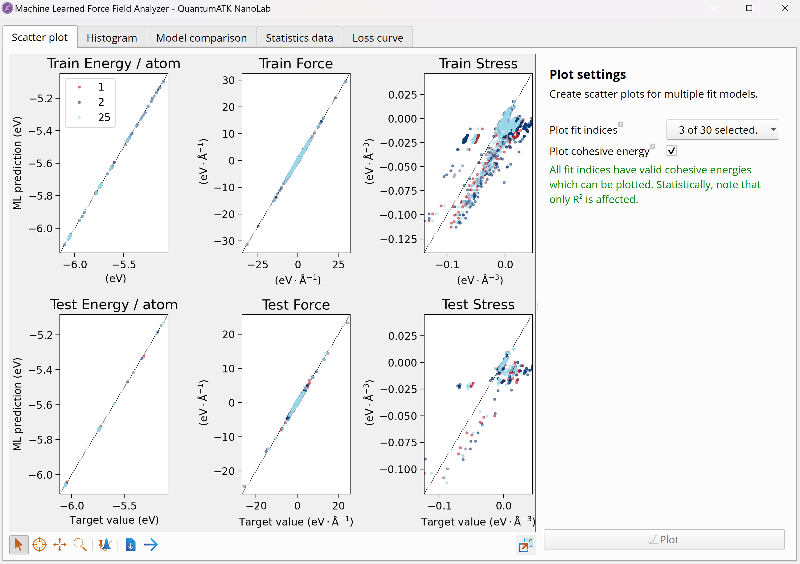
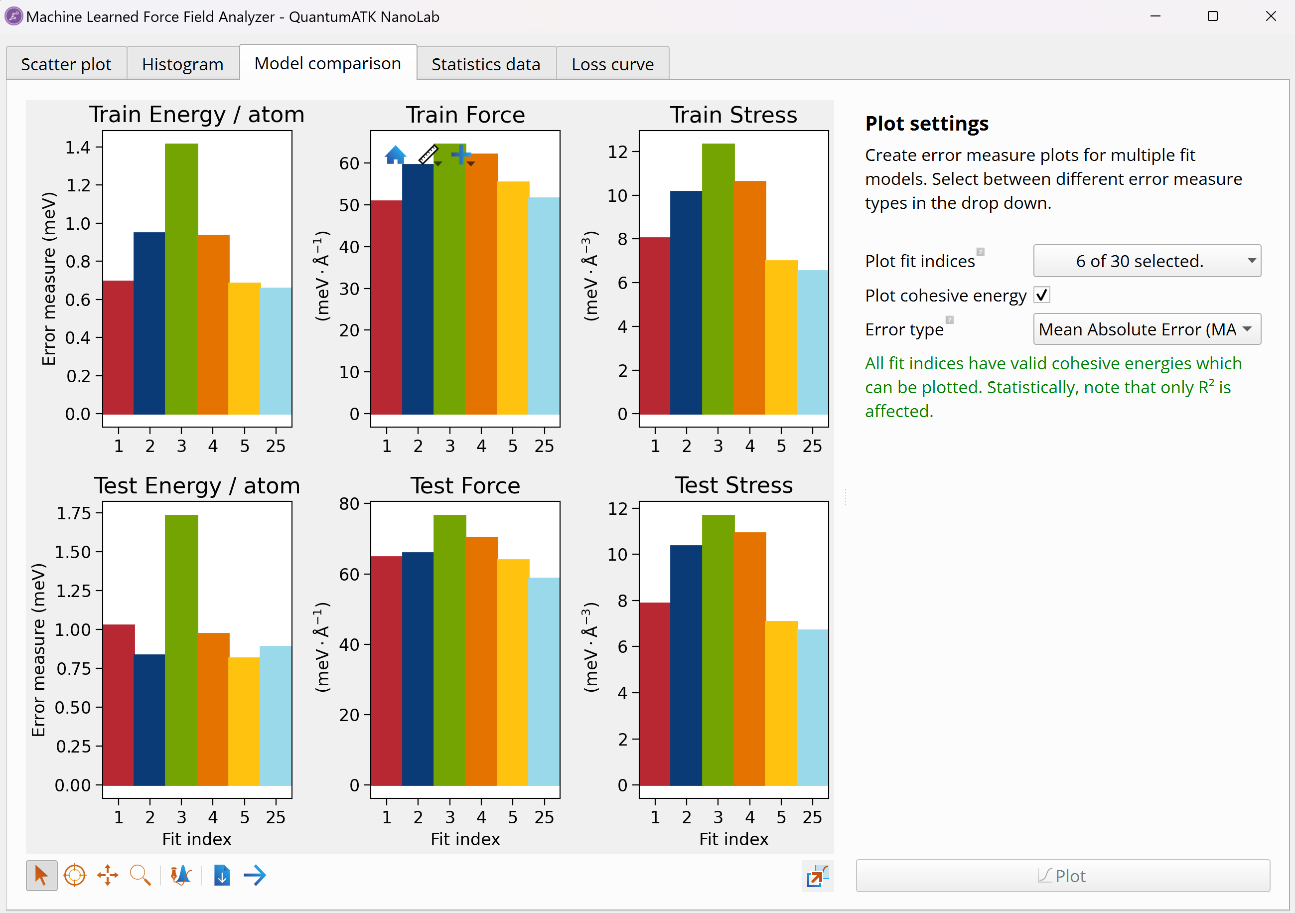
MTP fitting analysis to graphically inspect MAE, RMSE and r2
values for all 30 MTP fits. The MachineLearnedModelCollection
object can be opened with the Machine Learned Force Field Analyzer tool
in Nanolab. This tool allows you to see error histograms and scatter plots
of the predicted vs. reference values for energy, forces and stress for
each of the trained MTPs, as well as compare all trained models, visualize
their performance metrics, and identify the best model.
The above scatter plot compares the MTP predicted data (y-axis) and reference
DFT data (x-axis) for three different MTP fits. The energy, forces and stress
values are compared for both training and test sets and indicate high accuracy
of the trained MTP: the data points for energy and forces lie along the 45
degree line and for stress there are minor deviations, but overall good
correlation. In the model comparison plot, the MAE values for energy, forces
and stress for both training and test sets are shown for six example MTP fits.
Note
We recommend to look at the training configurations to aid potential
debugging. In case your production simulations with the trained MTP give
unexpected results, check if the training data set includes all the
important configurations that need to be included.
Look at c-am-TiSi-MTP-training-results_x.hdf5 to inspect Active
learning geometry optimization and melt-quench MD trajectories. Since we
started from 8 different initial amorphous configurations, we have 8
different .hdf5 files, where x=0-7.
Each .hdf5 file contains an alopt, md and md_3 objects,
which can be opened with the Movie tool
The alopt object is for inspecting the Active learning geometry
optimization trajectory along with the calculated energy and forces.
The md object is for the Active learning MD melting trajectory along
with the calculated temperature, energy, pressure, extrapolation grade,
etc. every 10 MD steps.
The md_3 object is for the Active learning MD cooling trajectory along
with the calculated temperature, energy, pressure, extrapolation grade,
etc. every 10 MD steps.
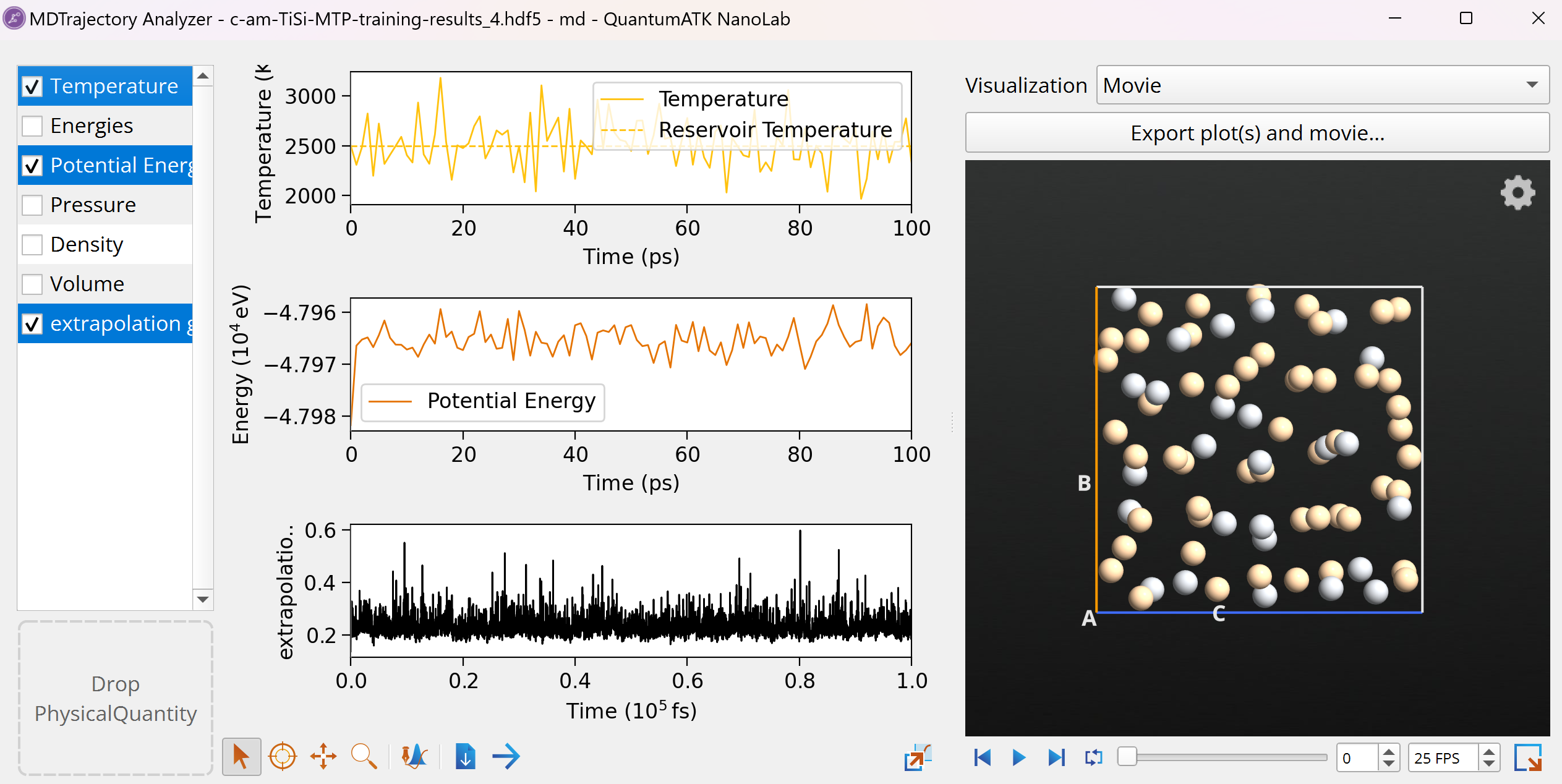
Open, e.g., the md object from the
c-am-TiSi-MTP-training-results_4.hdf5 with the Movie Tool to
inspect MD trajectory during the Active learning MD melting phase. Select
to also plot the extrapolation grade as a function of MD steps. You can
see that the extrapolation grade fluctuates during the MD, but at no point
does it exceed the candidate threshold of 1, thus no extrapolating
configurations are added to the training data set and the simulation
proceeds without interruption as it is deemed that the MTP is sufficiently
accurate for the visited configurations. In other cases, one might see
that the extrapolation grade exceeds the candidate threshold and then the
retrain threshold, which would lead to adding extrapolating configurations
to the training data set and re-starting Active learning MD with an
improved MTP.
Note
As shown in this tutorial, Active learning targets PES areas where the model
is uncertain and selects the extrapolating amorphous configurations (17 in
this case), for which to calculate DFT training data, thus minimizing the
number of expensive DFT calculations needed. Randomly sampling PES using MD
alone would require much longer simulation time scales, which would then
become computationally unfeasible if DFT is used for each MD step.
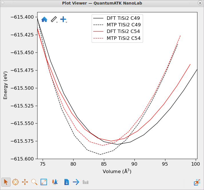
To validate the trained MTP for crystals, one can use the trained MTP to
calculate lattice constants and equation-of-state (EOS) for the relevant
crystal phases of titanium silicide, TiSi, TiSi2-C54 and
TiSi2-C49 and compare with the corresponding DFT results.
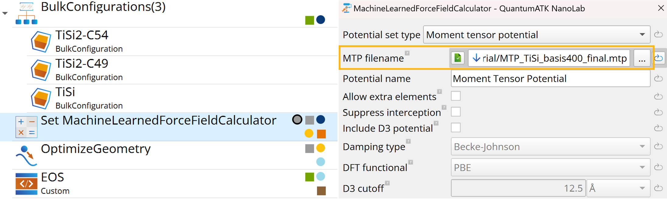
In the Set MachineLearnedForceFieldCalculator block, specify the location
and name of the final trained MTP, MTP_TiSi_basis400_final.mtp,
which will be used for the validation.
Run the workflows, and once the calculations of optimizing lattice constants
and obtaining EOS are finished, we are ready to analyze the results.
Download c-TiSi-DFT-EOS-results.hdf5 /
c-TiSi-MTP-EOS-results.hdf5 and then in the Data View window
select the optgeom, optgeom_1 and optgeom_2, which contain optimized
geometries of the three different crystal phases.
Right-click on optgeom, optgeom_1 and optgeom_2 objects to Open All
with Text Representation. Inspect and compare lattice constants of
optimized geometries obtained with the trained MTP and DFT. MTP gives good
agreement with DFT results (within 1-2%) for all crystal phases, as shown
in the table below.
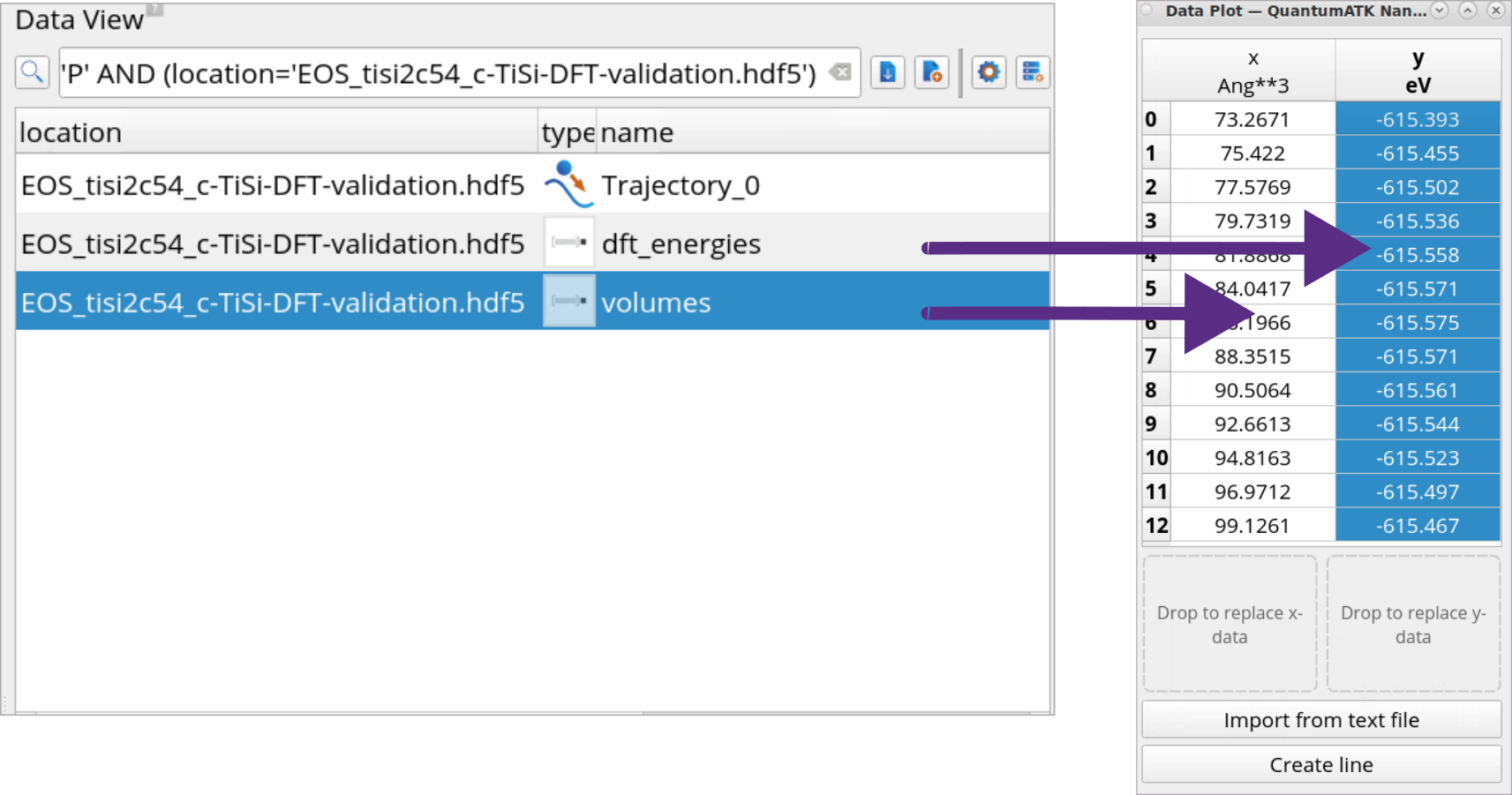
In Data View, find the Data Plot tool under Supplementary tools,
and then drag-and-drop volumes and dft_energies from the Data View
panel to the Data Plot tool x and y drop areas, respectively.
Click Create line to plot EOS for each crystal phase with DFT and MTP.
Repeat the steps 6 and 7 for each crystal phase with DFT and MTP for a
total of 6 plots.
Drag-and-drop the handle from one plot to another to
combine the plots into one.
Combined plots for TiSi2-C54 and TiSi2-C49 show that the
trained MTP reproduces the DFT trend, so that the TiSi2-C49
crystal phase is lower in energy than the TiSi2-C54 crystal phase
at the minimum.
To validate the trained MTP for amorphous structures, one can use the trained
MTP to run some short melt-quench MD simulations (50 ps melting and 50 ps
cooling) on, e.g., Ti26Si52, take some ~10 snapshots from
each and recalculate these with DFT and calculate the energy, forces and stress
RMSE between MTP and DFT.
In the Set MachineLearnedForceFieldCalculator block, specify the location
and name of the final trained MTP, MTP_TiSi_basis400_final.mtp,
which will be used for the validation.
Run the workflow and once the calculation is finished, we are ready to analyze
the results.
Open the am-TiSi-MTP-validation-results.log and at the end of
the file inspect the calculated energy, forces and stress RMSE between MTP
and DFT. Small RMSE values shown in the figure below indicate a good
accuracy of the trained MTP.
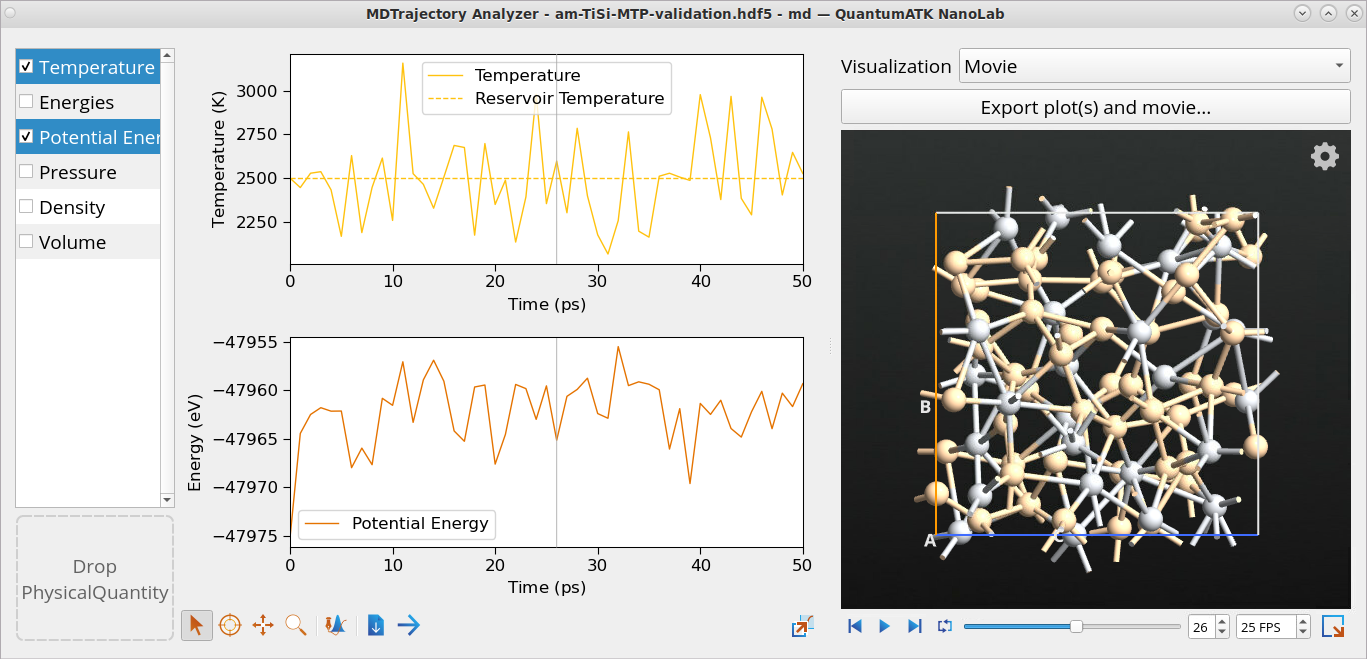
Open the md and md_2 objects from
am-TiSi-MTP-validation-results.hdf5 using the Movie Tool to
inspect MD trajectories from the 50 ps MD melting and from 50 ps cooling
simulations, respectively.
Note
It is recommended to check the MD trajectories with the trained MTP to
ensure that the trajectories look as expected and appear physical. In this
case, check that the amorphous configuration does not crystallize during the
cooling part of the simulation. In case of unexpected crystallization, one
can consider increasing the size (number of atoms) of the amorphous training
configurations and/or add additional amorphous configurations from Active
learning to the training data set.
In this introductory tutorial, you have learnt how to set up and analyze MTP
training and MTP quality validation calculations for crystal and amorphous
materials.
In order to adapt the introduced MTP training protocol for different geometries
(surfaces, interfaces, nanoparticles), stoichiometries, element composition and
other materials, you need to explicitly include relevant training data for such
structures.
Depending on the intended MTP application, consider also validating these
properties against the reference DFT values:
RDF and ADF for amorphous structures (it requires some long DFT-MD
simulations, which is expensive).
Experimental properties that are relevant for the application, if
available, but note that since the MTP is trained to reproduce DFT
results it can only be as accurate as the underlying DFT model.

 Workflow Builder.
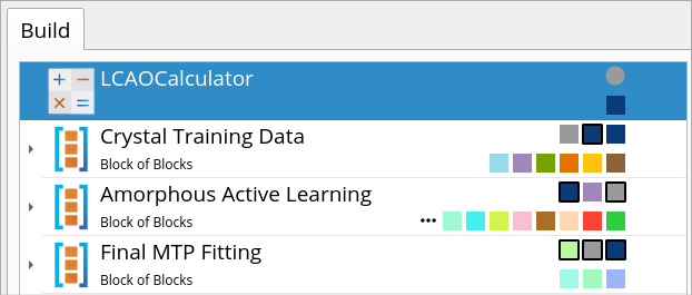
 LCAOCalculator block placed above
the three Blocks of Blocks is used for defining a reference DFT-LCAO
calculator (using the PBE xc-functional) that is used to calculate
training data (energy, forces and stress) throughout the MTP training
simulations.
LCAOCalculator block placed above
the three Blocks of Blocks is used for defining a reference DFT-LCAO
calculator (using the PBE xc-functional) that is used to calculate
training data (energy, forces and stress) throughout the MTP training
simulations.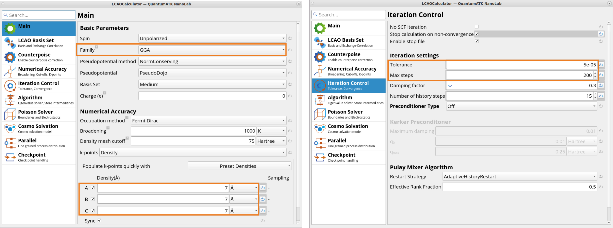

 Builder or from the Materials Project
database in the
Builder or from the Materials Project
database in the  Databases.
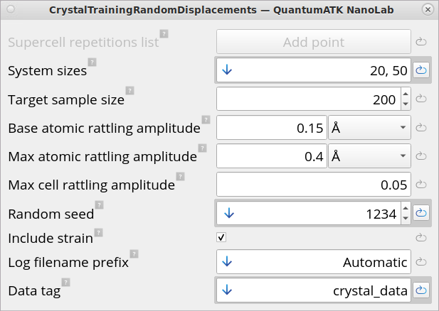
 Send content to other tools button
and choose Jobs as a script to send the workflow to the
Send content to other tools button
and choose Jobs as a script to send the workflow to the
 Jobs tool to submit this job on a local machine or a
remote cluster. It is recommended to use MPI parallelization for MTP
training simulations, as both training data calculations with DFT and MTP
fitting benefit from MPI parallelization.
Jobs tool to submit this job on a local machine or a
remote cluster. It is recommended to use MPI parallelization for MTP
training simulations, as both training data calculations with DFT and MTP
fitting benefit from MPI parallelization. Editor tool and then
sent to the
Editor tool and then
sent to the 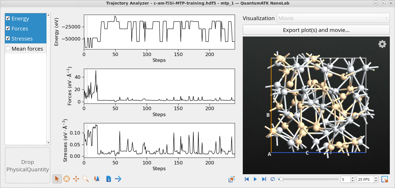
 handle from one plot to another to
combine the plots into one.
handle from one plot to another to
combine the plots into one.