Diffusion in Liquids from Molecular Dynamics Simulations
Version: P-2019.03
In this tutorial, you will learn how to calculate the atomic diffusion coefficient in liquid metals using molecular dynamics (MD) simulations. In general, an accurate measurement of the diffusion coefficient in liquids is a challenging task. The present tutorial demonstrates how the QuantumATK tools allow you to efficiently study this fundamental phenomenon in a straightforward manner on a computer instead.
We adopt classical molecular dynamics to be able to generate rather long MD trajectories of liquid copper. This is a computationally efficient approach to obtain statistically meaningful averages of the physical quantities needed for calculating the diffusion coefficient of a single Cu atom in this liquid metal. The entire MD procedure is divided into three major steps:
heating crystalline copper to above its melting point,
annealing liquid copper at high temperature to bring the system to equilibrium,
further annealing of this equilibrated liquid copper to get more statistical data for accurate calculation of the atomic diffusion coefficient, using the time-dependent mean-square displacement derived from the corresponding MD trajectory.

Theory
Diffusion in liquid metals differs from atomic diffusion in solids, as it takes place at a much shorter time scale, allowing for a brute force approach based on molecular dynamics simulations to calculate an atomic diffusion coefficient, denoted \(D\). Knowing this fundamental physical quantity is needed to understand liquid dynamics, as well as many other related phenomena, such as nucleation and crystal growth. Unfortunately, experimental diffusion data for liquids are often rather inaccurate for various reasons [1]. Instead, liquid diffusion can be rather accurately studied theoretically as demonstrated in this tutorial.
Tip
If you are interested in atomic diffusion in solids, please refer to the following two tutorials on Boron diffusion in bulk silicon and Modeling Vacancy Diffusion in Si0.5 Ge0.5 with AKMC as studying diffusion in solids usually requires a more sophisticated computational approach compared to the molecular dynamics approach.
Given that the MD simulation of the equilibrated liquid has been run for time \(T_{\rm MD}\), the diffusion coefficient, \(D\), can then be expressed in terms of the mean-square displacement of atoms in this MD run
where \(\left\langle X^{2}(t) \right\rangle\) is the mean-square displacement of Cu atoms in liquid copper, calculated at the observation time \(t\)
and \(N_{\rm at}\) is the total number of Cu atoms in the supercell, and \({\bf r}_{j}(t^{\prime}+t)\) and \({\bf r}_{j}(t^{\prime})\), where \(j \in [1,\ldots,N_{\rm at}]\), are atomic position coordinates at time \(t^{\prime}+t\) and \(t^{\prime}\), respectively. In this tutorial, \(t\) is the time interval of observation that is adopted to extract the atomic diffusion coefficient from the time-dependent mean-square displacement, \(\left\langle X^{2}(t) \right\rangle\), assuming that \(\left\langle X^{2}(t) \right\rangle\) shows a linear behavior with respect to \(t\). This observation time \(t\) cannot exceed the total time \(T_{\rm MD}\) of the MD simulation of liquid. The mean-square displacement may become quite noisy, not showing a linear dependence with respect to the time interval \(t\) for the values of \(t\) close to \(T_{\rm MD}\). In some cases, only those values of \(t\) that are much smaller than the simulation time, i.e., when \(\, \, t\ll T_{\rm MD}\), allow for accurate estimates of the diffusion coefficient from the linear fit of \(\left\langle X^{2}(t) \right\rangle\).
Strictly speaking, the formula given in the previous paragraph defines the self-diffusion coefficient of liquid copper. That is the atomic diffusion coefficient averaged over all the copper atoms in the liquid. This ensemble averaging is possible in this case because all these copper atoms are assumed to be identical, having the same atomic mass and other physical characteristics that may affect diffusion of atoms. If a foreign (impurity) atom or a copper isotope with a different atomic mass was introduced in liquid copper, we would then have an additional diffusion process, which is diffusion of this foreign atom in liquid copper. To quantify this process, we can calculate the atomic diffusion coefficient, \(D_{\rm imp}\), of this single atom as follows
where the individual atom trajectory \(r_{\rm imp}(t)\) is taken from the MD trajectory of the entire system of many atoms.
One should bear in mind that diffusion properties of materials depend on the temperature, and that also holds true for the atomic diffusion coefficient. In this tutorial, we will study liquid copper at T=2000 K, which is a temperature well above the melting point of crystalline copper.
Computational Procedure
Building a Copper Supercell Structure
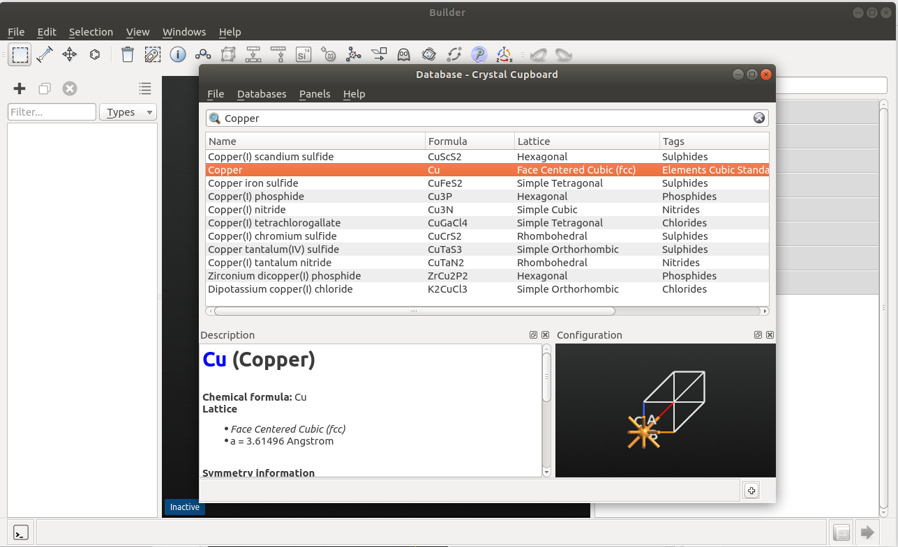
Open the Builder
 and add a face-centered crystal structure of Copper from Database to the Stash.
In Bulk Tools, choose Supercell and click on Conventional.
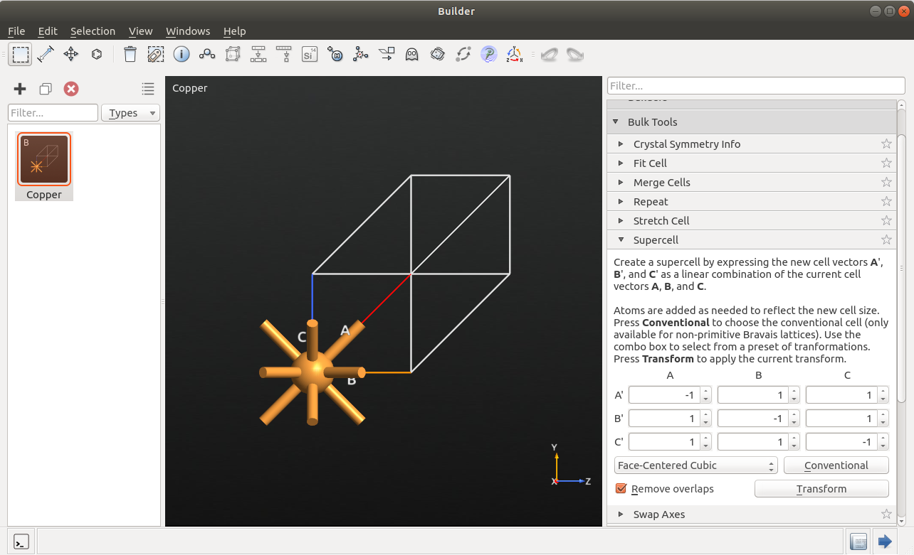
Then click on Transform to convert the primitive cell of bulk copper with 1 Cu atom to the conventional unit cell with 4 Cu atoms.
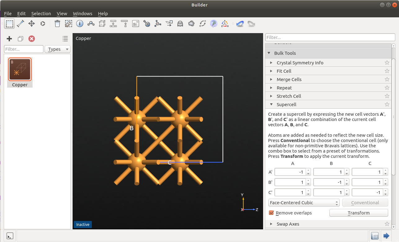
In Bulk Tools, choose Repeat and set the repetition of the conventional unit cell along the A, B, and C axes to 6.
Click on Apply to create a 6x6x6 cubic supercell of bulk copper, which is the initial structure for MD simulations.
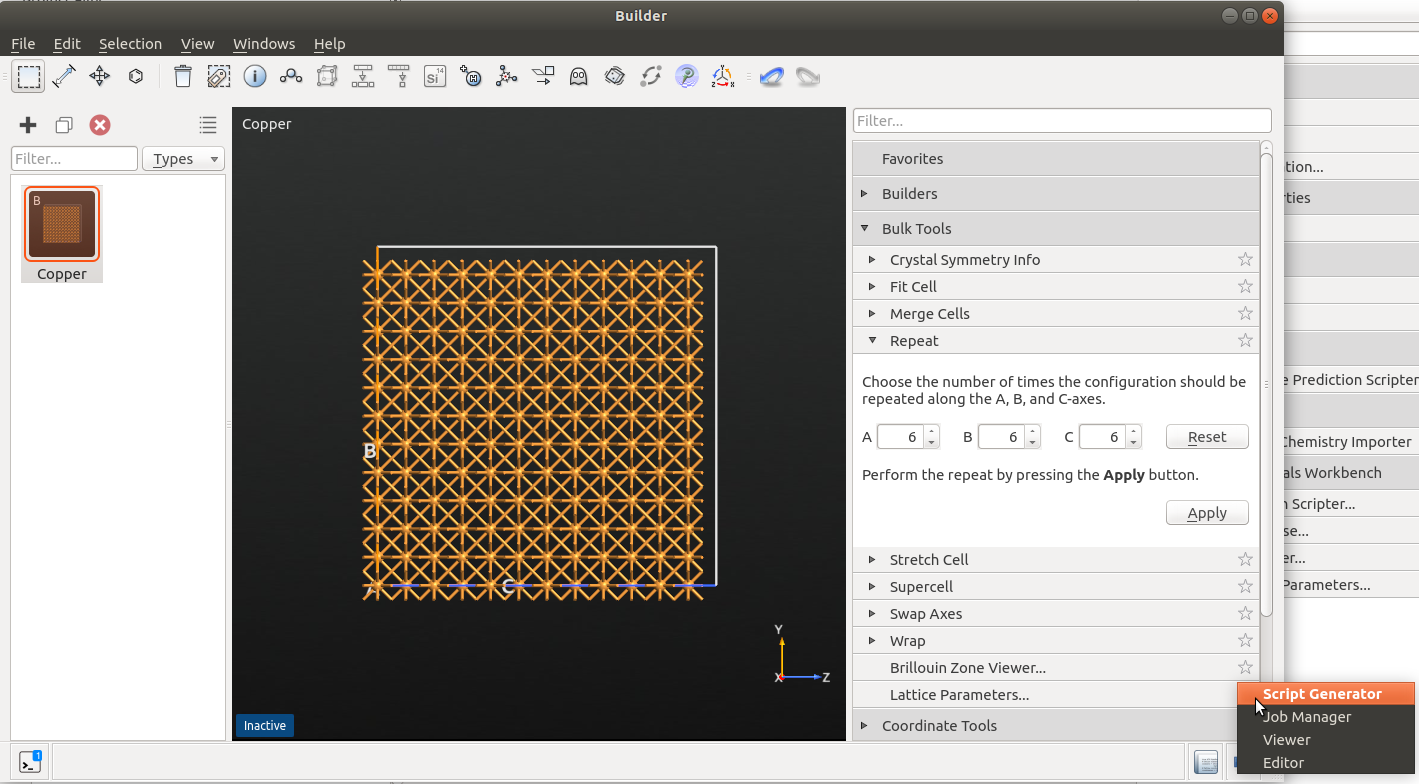
Send the copper supercell structure to the Script Generator
 with the Send To icon
  .
.
Setting up MD Simulations in the Scripter
Add a
 .
.
Note
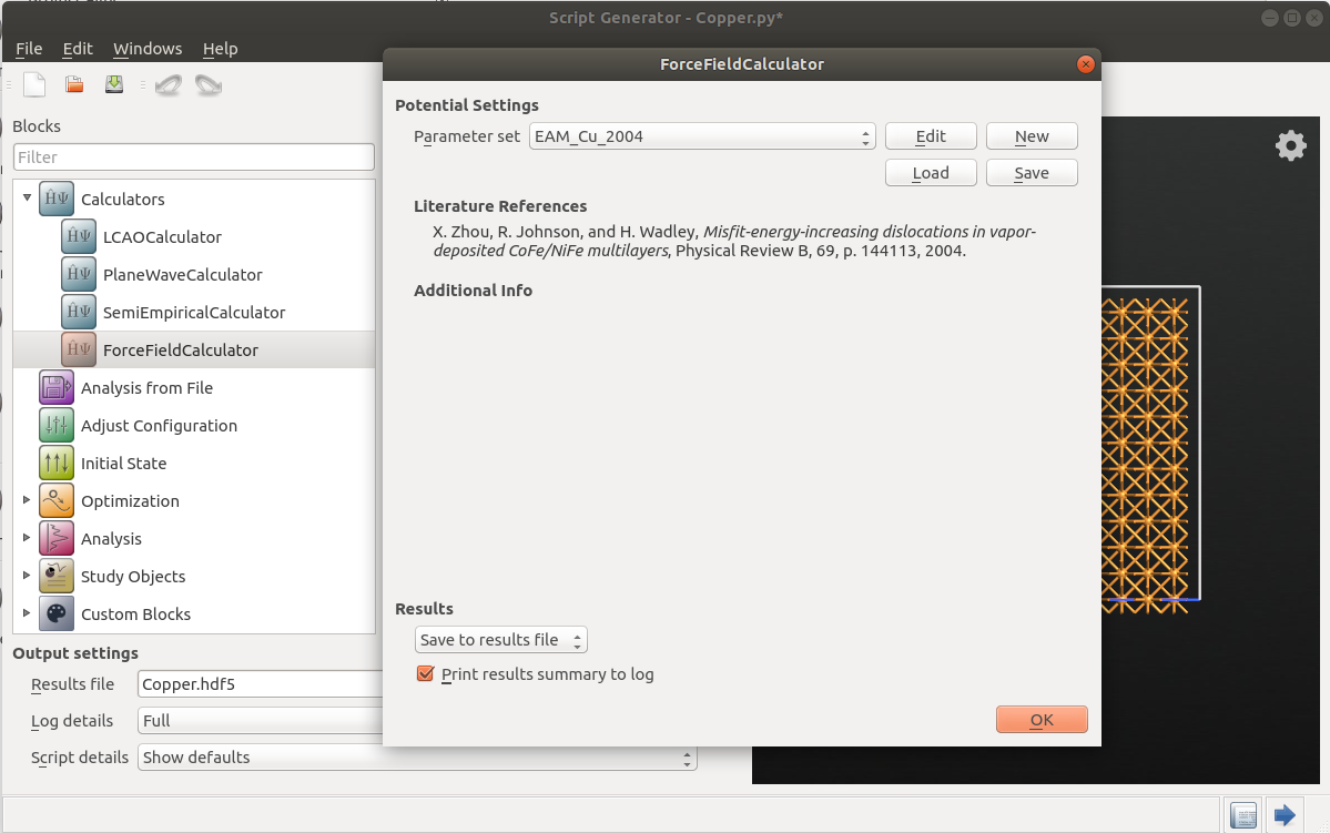
For QuantumATK-versions older than 2017, the ATK-ForceField calculator can be found under the name ATK-Classical.
In the Potential Settings, set the classical potential in Parameter set to EAM_Cu_2004 [2].
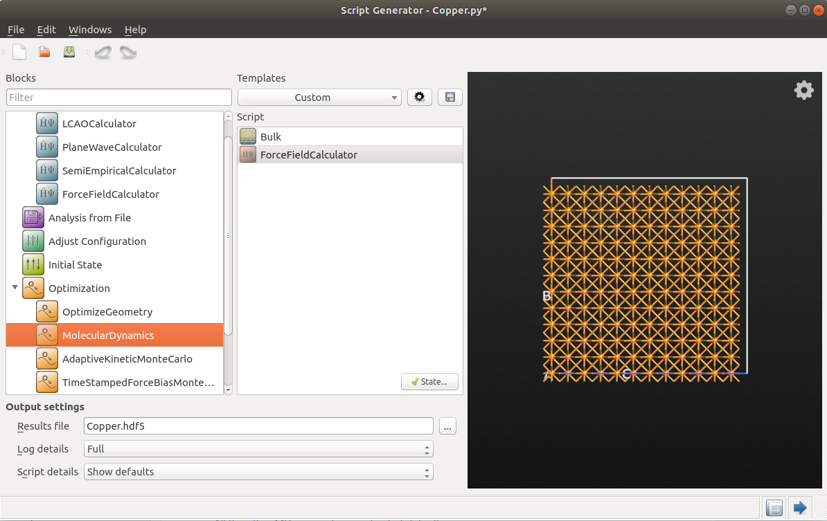
Add an object to the Script to set up the first step of the MD procedure, which is heating crystalline copper above its melting point.
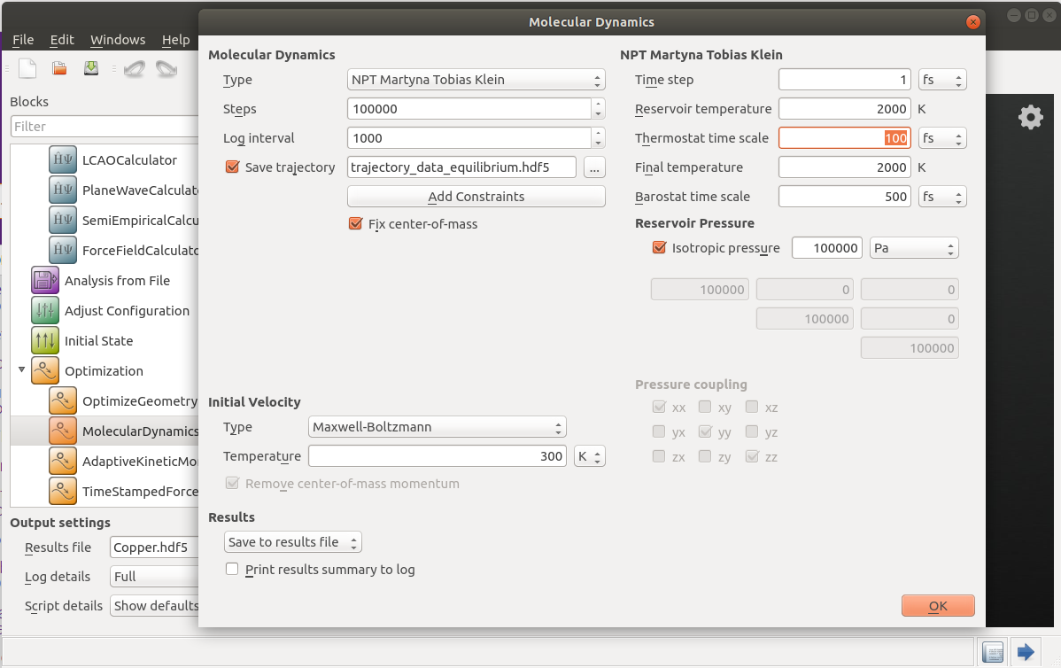
Set the computational parameters for MolecularDynamics to heat up the supercell structure of crystalline copper from 1000 to 2000 K, using an NPT barostat. This procedure allows us to increase the temperature of the system gradually above its melting point. It means that the ordered solid will eventually become a liquid, which only exhibits a short-range order as demonstrated using the radial distribution function (RDF) in the Analysis section.
Set Molecular Dynamics Type to NPT Martyna Tobias Klein, Steps to 100000, Log interval to 1000, and Save trajectory to the
trajectory_heating.hdf5file.Set Initial Velocity Type to Maxwell-Boltzmann, and Temperature to 1000 K.
In the NPT Martyna Tobias Klein barostat settings, set Reservoir temperature to 1000 K, and Final temperature to 2000 K.
All the other MD parameters are kept at default.

Add a second object to the script to set up the second step of the MD procedure, which is annealing liquid copper to bring the system to equilibrium.
We should set the computational parameters for MolecularDynamics to equilibrate the supercell structure of liquid copper at the constant temperature 2000 K, using an NPT barostat. This step is needed to eliminate any memory effect of the initial copper structure (solid copper) on the physical properties of liquid copper obtained from this particular initial structure.
Set Molecular Dynamics Type to NPT Martyna Tobias Klein, Steps to 100000, Log interval to 1000, and Save trajectory to the
trajectory_equilibrating.hdf5file.Set Initial Velocity Type to Maxwell-Boltzmann, and Temperature to 2000 K.
In the NPT Martyna Tobias Klein barostat settings, set Reservoir temperature and Final temperature to 2000 K.
All the other MD parameters are kept at default.

Add a third object to the script to set up the third step of the MD procedure to collect sufficient statistical data for calculating the self-diffusion coefficient of liquid copper.
Set the computational parameters for MolecularDynamics to run the MD simulation for the supercell structure of equilibrated liquid copper at the constant temperature 2000 K, using an NPT barostat. In this step, we aim at collecting a good statistical data (a set of MD frames) for calculating atomic diffusion coefficient of liquid copper.
Set Molecular Dynamics Type to NPT Martyna Tobias Klein, Steps to 100000, Log interval to 1000, and Save trajectory to the
trajectory_data_equilibrium.hdf5file.Set Initial Velocity Type to ConfigurationVelocities, so that the velocities from the previous (second) MD run will be used as initial velocities for this (third) MD simulation.
In the NPT Martyna Tobias Klein barostat settings, set Reservoir temperature and Final temperature to 2000 K.
All the other MD parameters are kept at default.
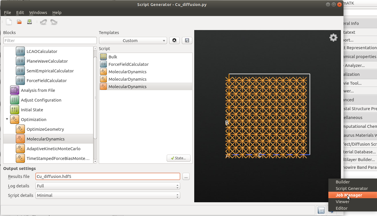
In Output settings, rename Results file to
Cu_diffusion.hdf5, and save the Script toCu_diffusion.py.

Send the job to the Job Manager
 .
.
Depending on your machine, it will take about half an hour to do the classical MD simulations for the supercell structure with 864 copper atoms adopted in this tutorial.
Download the scripts here: Cu_diffusion.py and analysis.py.
Analysis
Self-diffusion of Liquid Copper
Once the calculations are done, the requested HDF5 data files should appear in the QuantumATK Project Files list, and their contents should be visible on the LabFloor.
Select the trajectory named
trajectory_heating.hdf5and open the Movie Tool from the right-hand plugins bar.
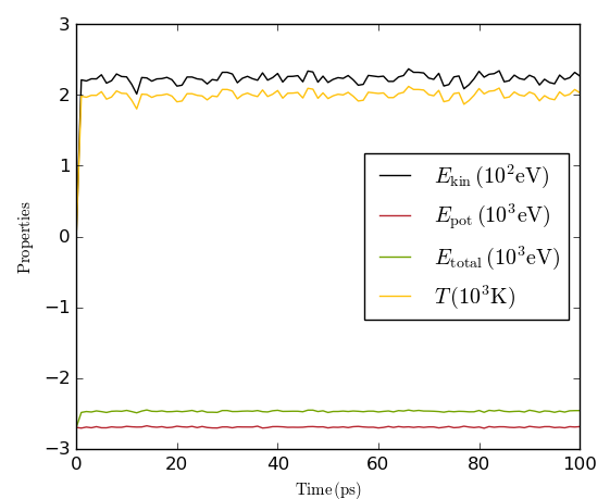
The left-hand plot shows the time-evolution of the MD quantities: kinetic energy, potential energy, total energy, and temperature, all as a function of MD simulation time. On the right you can see a movie of the MD trajectory.
Use mouse right-click to tick the option Wrap bulk atoms, and then click on the
 icon to start the movie.
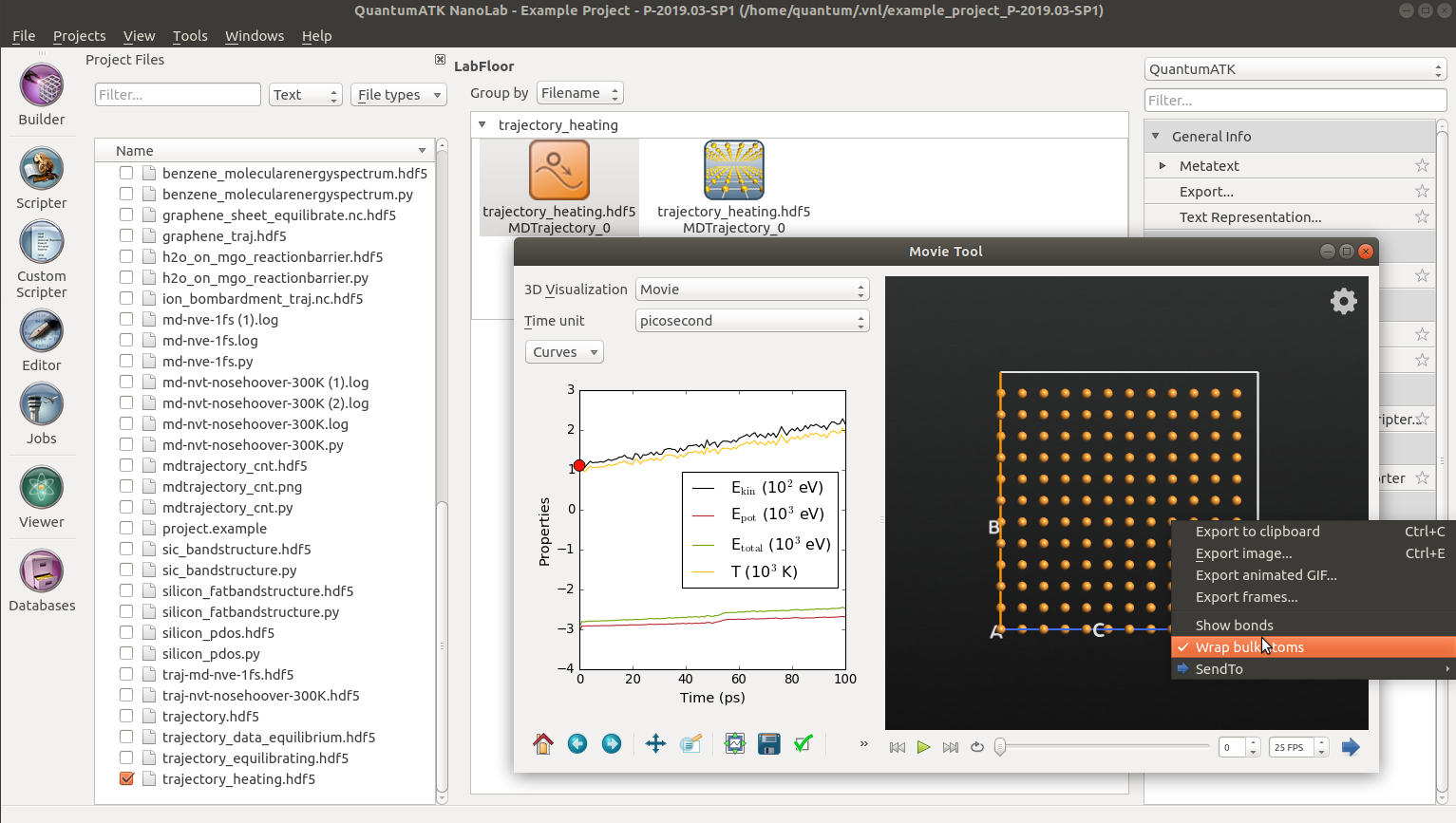
As shown in the animation of the MD trajectory, the average velocity of the copper atoms increases at elevated temperatures, and then the phase transition from the crystalline to liquid copper occurs about half-way through the heating MD run.
Tip
You can easily save such an animated GIF file yourself: Right-click the movie and select Export animated GIF.
You can also use the Movie Tool to inspect the trajectory for the equilibration MD run, trajectory_equilibrating.hdf5. Note that the temperature and energy are fairly constant throughout the equilibration of the system:
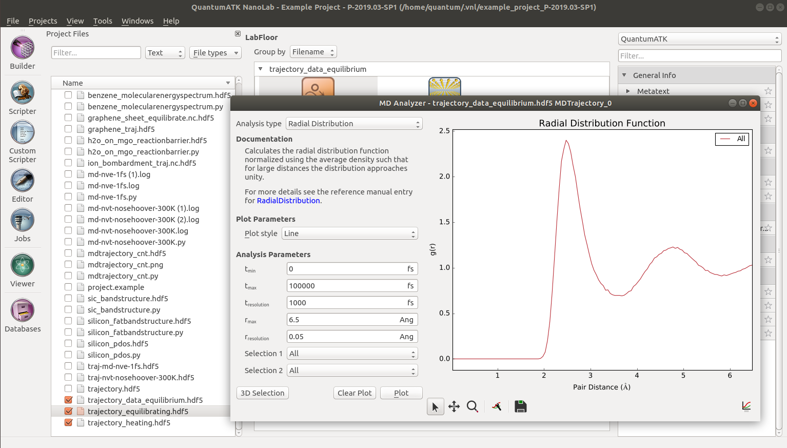
As mentioned in the Computational procedure section, an ordered solid transforms into a liquid phase with a short-range order preserved upon melting. To demonstrate that liquid copper exhibits some structural ordering, select the final MD trajectory, trajectory_data_equilibrium.hdf5, and open the MD Analyzer from the right-hand plugins bar. Select Radial Distribution in the drop-down menu, and click on Plot to generate a plot of the radial distribution function \(g(r)\) for the liquid copper. The distribution function shows a pronounced peak at 2.5 Å, indicating that this is the dominant nearest-neighbor distance between atoms in the liquid copper. This value is comparable to the nearest-neighbor bond distance of 2.55 Å in crystalline copper at room temperature, suggesting that there still exists some short-range order in the liquid phase of copper.
As described in the Theory section, the diffusion coefficient is related to the mean-square displacement (MSD) of the Cu atoms as the final MD simulation progresses. You can plot the MSD using the MD Analyzer: Select Mean Square Displacement as the quantity to be plotted, and then click on Plot.
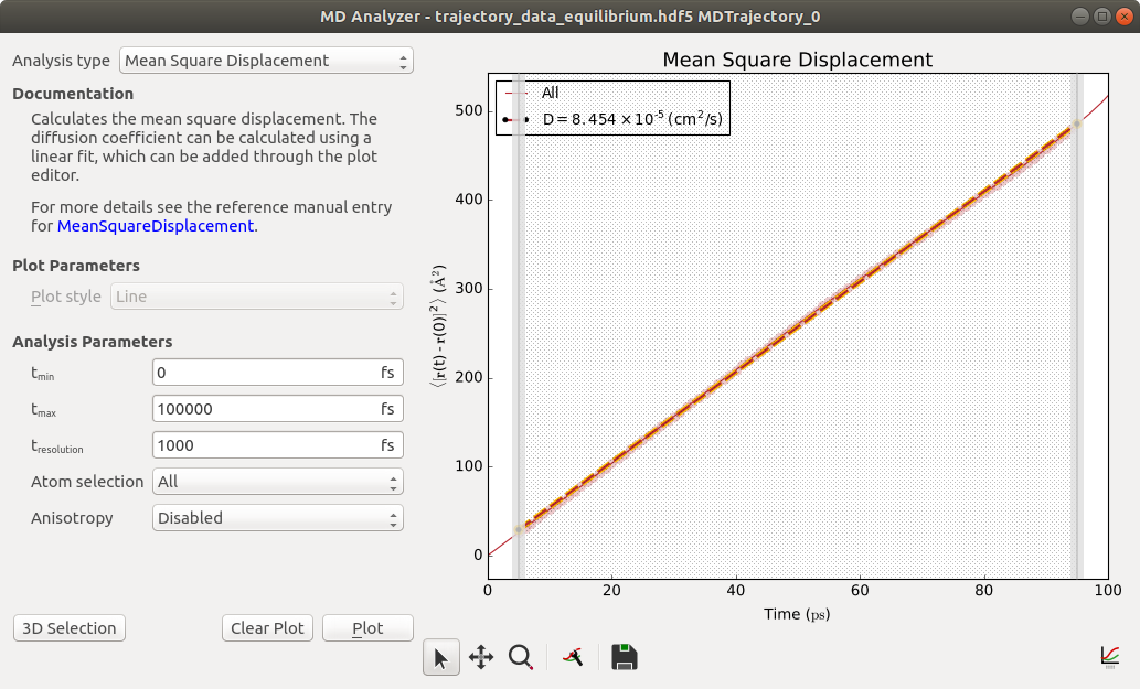
The MSD increases linearly with simulation time, and all you need to compute the diffusion coefficient is the slope of the line. Right-click on the line, select “Add fit”, and click “Polynomial fit”. Close the Plot editor.
The atomic diffusion coefficient in liquid copper calculated at 2000 K is 0.85 Å2/ps.
Diffusion of a Single Atom in Liquid Copper
To demonstrate how the diffusion coefficient, \(D_{\rm imp}\), of an individual atom in liquid can be obtained within the framework of the MD approach, we will look at the diffusion of a single copper atom in the liquid copper, pretending that this (randomly-chosen) atom differs from all the other copper atoms in the system. In this particular case, one would expect that the value of the atomic diffusion coefficient for this individual atom should be close to the self-diffusion coefficient value of liquid copper.
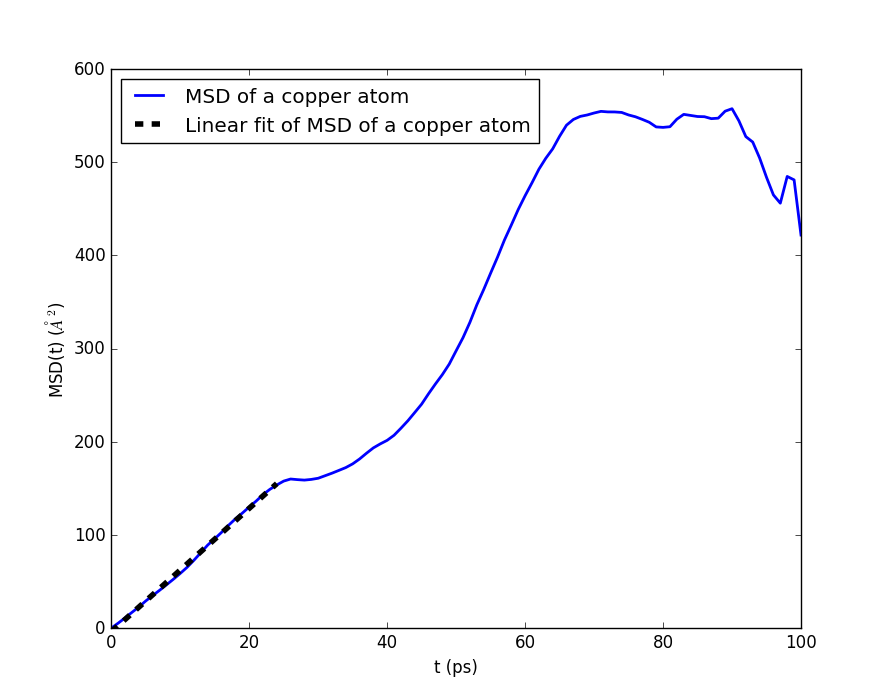
The MD trajectory that has already been obtained for liquid copper can be directly adopted for calculating atomic diffusion of a single copper atom. The MSD of a single atom also increases linearly with simulation time, at least on the short-time scale as seen in the figure given below, and all you need to compute the diffusion coefficient is the slope of the line.
Use the script analysis_single_atom.py for computing the diffusion coefficient. The
content of the script is shown below. The script takes as an argument the name of the HDF5 file
trajectory_data_equilibrium.hdf5 from which it extracts the MD trajectory of a single copper atom (atom #7 as chosen in the script) in the equilibrated liquid copper, then uses the built-in function MeanSquareDisplacement() to calculate the MSD of the copper atom #7, and uses NumPy to do the linear fitting. Finally, a plot is produced using pylab.
# Get the name of the MD trajectory (hdf5) file given in the system arguments
filename = sys.argv[1]
#filename = 'trajectory_data_equilibrium.hdf5'

# Get the frames of the MD trajectory from the file
md_trajectory = nlread(filename)[-1]

# Get Mean Square Displacement (MSD) for a single Cu atom (#7) from the MD trajectory
msd = MeanSquareDisplacement(md_trajectory,atom_selection=[7])

# Get the times in ps and the MSD values in Ang**2.
t        = msd.times().inUnitsOf(ps)
msd_data = msd.data().inUnitsOf(Angstrom**2)

# Fit the slope of the MSD to estimate the diffusion coefficient.
# If you discover non-linear behavior at small times, you should then discard this initial part in the fit.
for i in range(10,110,10):
  first_image = 0
  a = numpy.polyfit(t[first_image:i], msd_data[first_image:i], deg=1)
  print(i, a[0]/6)

# Setting the endpoint to 25 is based on a visual inspection of the plot for MSD(t).
# Note that this kind of plots may have some noise for large time-values.
endpoint = 25
a = numpy.polyfit(t[first_image:endpoint], msd_data[first_image:endpoint], deg=1)
line_fit = numpy.poly1d(a)

# Calculate the diffusion coefficient of the copper atom #7 in Ang**2/ps.
diffusion_coefficient = a[0]/6.0
print('Diffusion coefficient for a single atom in liquid copper at T=2000K is: ',diffusion_coefficient, ' Ang**2/ps')

# Plot the data using pylab.
import pylab

pylab.plot(t, msd_data, linewidth=2,label='MSD of a copper atom')
pylab.plot(t[first_image:endpoint], line_fit(t[first_image:endpoint]), linewidth=4,color='k', linestyle='--', label='Linear fit of MSD of a copper atom')
pylab.xlabel('t (ps)')
pylab.ylabel('MSD(t) ($\AA^{2}$)')
pylab.ylim(0,600)
pylab.legend(loc='upper left')

pylab.show()
Download the script and execute it from the command line. The calculated diffusion coefficient of a single atom will be printed at the end of the logging output:
$ atkpython analysis_single_atom.py trajectory_data_equilium.hdf5
...
...
...
Diffusion coefficient for a single atom in liquid copper at T=2000K: 1.10459718032 Ang**2/ps
Tip
This python script used for the analysis can also be executed from the Job Manager, i.e., without using the command line. For that, replace filename = sysargv[1] with filename = ‘trajectory_data_equilibrium.hdf5’ in the downloaded analysis_single_atom.py script, save it, and send it to the Job Manager to execute it as a regular QuantumATK job.
The diffusion coefficient of a single atom in liquid copper calculated at 2000 K is found to be 1.10 Å2/ps in this case. As expected, this value is comparable to that of the self-diffusion coefficient of liquid copper, 0.89 Å2/ps. The difference between these two calculated coefficients originates from the fact that we have done ensemble-averaging over all the copper atoms in liquid to calculate the self-diffusion coefficient, \(D\), whereas there is only one data point at a given time, \(t\), for calculation of the atomic diffusion coefficient, \(D_{\rm imp}\). So, we may need to run MD simulations for much longer time (\(T_{\rm MD}\)) to more accurately calculate the self-diffusion coefficient of liquid copper from the MD trajectory of a single copper atom. This longer MD trajectory should allow us to get better statistics and increase the observation time interval (\(t\)) where the mean-square displacement exhibits a linear time dependence. The linear region in the following figure, which shows the time-dependent mean-square displacement, is then expected to increase from \(t=25\) ps to a larger observation time value.
Note
When analyzing only a single atom for this amount of time, the statistics are not sufficient for obtaining the diffusion constant. If you want the diffusion constant from a single atom, the simulation needs to run much longer than if the averaging is done over many atoms.
Temperature Dependence of Diffusion Coefficient
As an exercise, you may repeat all the steps of the MD procedure to obtain the MD trajectory of liquid copper equilibrated at T=1620 K, and then calculate the self-diffusion coefficient from this MD trajectory. You will find that this physical quantity calculated without any adjustable parameters, i.e., calculated from first-principles, agrees very well with the experimental value of 0.52 Å2/ps measured for liquid copper at T=1620 K. The smaller diffusion coefficient value at 1620 K compared to that at 2000 K suggests that the self-diffusion coefficient decreases upon lowering the temperature of liquid, as expected.
References