Vibrational modes and Vibration Visualizer
In this tutorial you will study the vibrational properties of nanoscale systems using the VibrationalMode analysis object and the Vibration Visualizer plugin. Two systems are investigated:
Monolayer MoS2.
A nanophononic metamaterial
Note
Calculation of vibrational properties relies on the dynamical matrix of the configuration, which describes the force response on all atoms due to out-of-equilibrium displacements of all other atoms.
MoS2 monolayer
Generate the MoS2 structure
Open the  Builder, and do the following:
Use the Database plugin via and locate molybdenite. Add it to the Stash.
Use the mouse to select and delete the 3 atoms to the right in the cell. This leaves a single layer of MoS2.
Open and change the z direction to 25 Å.

Center the structure using .
Send the structure to the
 Script Generator
by using the
Script Generator
by using the  icon. The next step is to create the script to optimize the structure.
Optimize the MoS2 structure
Add
 New Calculator and
  OptimizeGeometry blocks.
In New Calculator, use the ATK-ForceField engine and in particular the “StillingerWebber_MoS_2013” potential`.
Note
For QuantumATK-versions older than 2017, the ATK-ForceField calculator can be found under the name ATK-Classical.

In OptimizeGeometry, reduce the force and stress tolerance to 0.001 eV/Å and 0.001 eV/Å3, click OK and save the script before running the optimization.

Save the script as
mos2_relax.py. Run the script by sending it to the Job Manager, or from a terminal with the command
$ atkpython mos2_relax.py > mos2_relax.out
An example script mos2_relax.py is available to download.
Note
In the case of monolayer, the potential agrees exactly with Ref. [1]. However, the Lennard-Jones potential reported in the reference for the inter-layer coupling has not yet been implemented.
Phonon band structure and density of states
The phonon band structure and the phonon density of states are now easily obtained:
Drop the optimized MoS2
BulkConfigurationonto the Scripter and add a New Calculator by double clicking it.Change the default output file to
mos2_phonons.nc.Check if the calculator is set to ATK-ForceField.
Add the
 and
analysis objects.
and
analysis objects.Note that the
was automatically added also.Open the DynamicalMatrix block and select and set the repeats to (21,21,1).

Open PhononBandstructure and set “Points pr. segment” to 400 and set the Brillouin zone route to the sequence [G, M, K, G].
In , untick “Sync” and set the q-point sampling to (99, 99, 1).

Run calculation and analyze results
Run the calculation. Once finished, the LabFloor should contain the PhononBandstructure and PhononDensityOfStates objects:
 PhononBandstructure
 PhononDensityOfStates
Inspect the phonon band structure and density of states using the Bandstructure Analyzer and 2D Plot tools. The results are in complete agreement with literature data [2].

Vibrational Modes
To visualize the vibrational modes, a simple post-processing is sufficient:
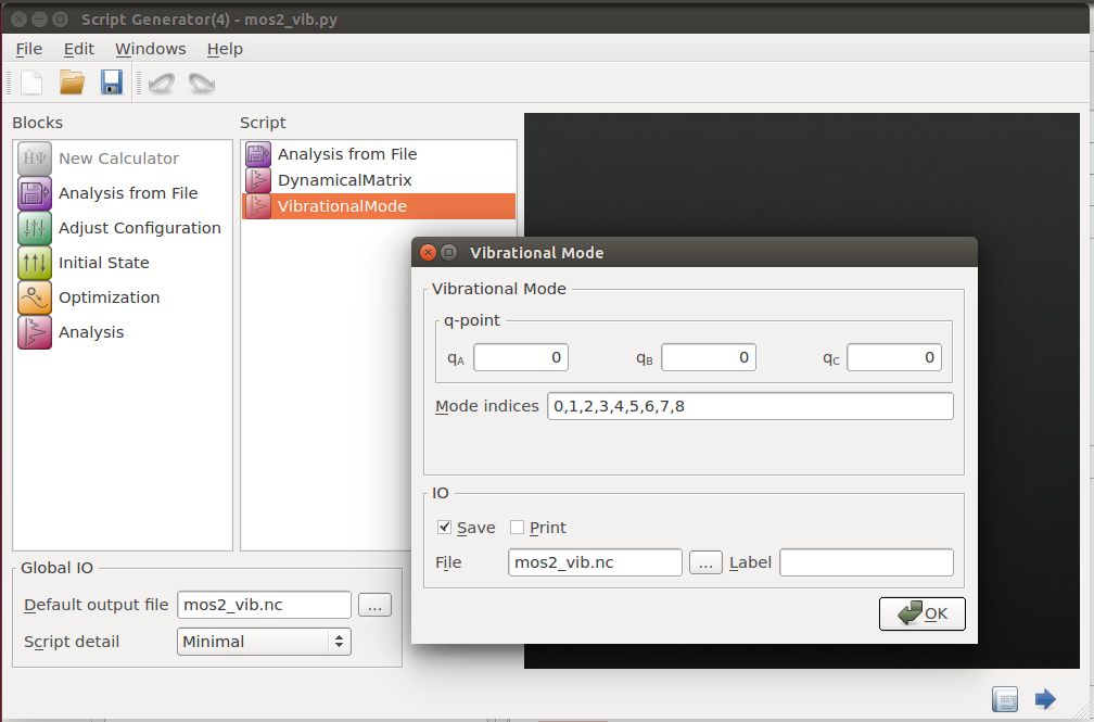
Open the
Script Generator and do the following:Add an
 Analysis from File block, double
click to open it, select the output file
Analysis from File block, double
click to open it, select the output file mos2_phonons.nc, and choose the subject id as “gID000”.Add a
analysis object
and select the q-point coordinates and mode indices of interest.
The script will recalculate the dynamical matrix, which is
inconvenient. To reuse the already calculated dynamical matrix, send
the script to the editor and change the line defining the dynamical
matrix such that it reads object “gID001” from the file mos2_phonons.nc.
 1# -------------------------------------------------------------
 2# Analysis from File
 3# -------------------------------------------------------------
 4configuration = nlread('mos2_phonons.nc', object_id='gID000')[0]
 5
 6# -------------------------------------------------------------
 7# Dynamical Matrix
 8# -------------------------------------------------------------
 9dynamical_matrix = nlread('mos2_phonons.nc', object_id='gID001')[0]
10
11# -------------------------------------------------------------
12# Vibrational Mode
13# -------------------------------------------------------------
14vibrational_mode = VibrationalMode(
15    configuration=configuration,
16    dynamical_matrix=dynamical_matrix,
17    kpoint_fractional=[0, 0, 0],
18    mode_indices=[0,1,2,3,4,5,6,7,8]
19    )
20nlsave('mos2_vib.nc', vibrational_mode)
Execute the script, and when the calculation is complete you will find the VibrationalMode object on the LabFloor:
 VibrationalMode
Select it and open it by clicking the Vibration Visualizer plugin. You can then visualize the vibrational mode as an animation.

Once you are done with the settings you can right click on the plot to export as a picture or as an animated gif. The two animated gifs below illustrate mode 4 at Γ (276.87 cm-1) and at M (252.32 cm-1), respectively.

You can play around with the Vibration Visualizer and compare the results with the literatures values in [2][3][4].
Nanophononic metamaterials
Another great example of the vibrational mode analysis is simulation of a nanophononic metamaterial. Bruce L. Davis and Mahmoud I. Hussein recently reported that specific vibrational modes of pillared silicon thin films will strongly suppress the thermal conductivity of the films due to the local resonance [5]. Let’s study the vibrational feature of the structure using ATK:
Calculation Setup
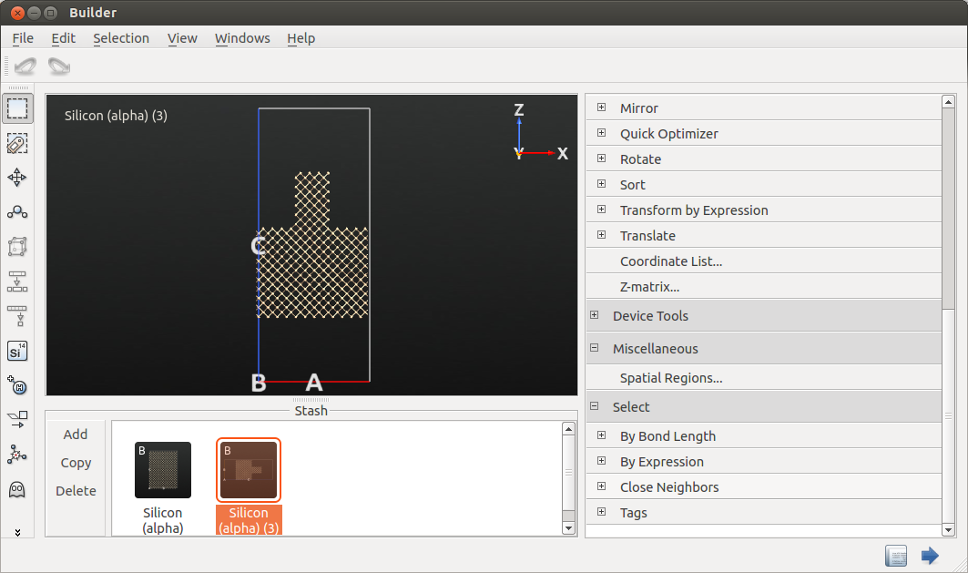
Open the Builder and do the following:
Use to add “Silicon (alpha)” to the Stash.
Transform the primitive cell into the conventional cell using .

Use the to repeat the structure 6x6x8 times to create a configuration with 2304 silicon atoms.
Use the Selection Tools, in particular , to cut out a pillared structure.
Tip
The expression “z > 20 and x < 10” will select one particular part of the configuration that could then be removed by .
Adjust the structure by increasing the lattice vector and pillar pointing direction to create a vacuum region above and below the pillared film.
Send the configuration to the Scripter and add a Calculator, a PhononBandstructure analysis object and two VibrationalMode objects.
Setup the calculator to use ATK-ForceField.
Tip
You can leave the settings in DynamicalMatrix by defaults when calculating a 3D structure.
Open PhononBandstructure and
set “Points pr. segment” to 100,;
set “Number of bands” to 50;
set the Brillouin zone route to [G, X].
Edit both VibrationalMode objects such as to calculate the vibrational modes in the Γ point (0, 0, 0) and in the X point (0.5, 0, 0) and select mode indices [0,1,2,3,4,5,6,7,8] in both objects.
Run the calculation. It will take a while for a single CPU core, but will be very efficient if the job is parallelized.
Results
Plot the calculated phonon bandstructure, and compare it with the phonon bandstructure of a uniform film. You can see that the array of pillars introduces a series of localized states (without dispersion), which are the states that lower the thermal conductivity of the silicon film, as explained in Ref. [5].
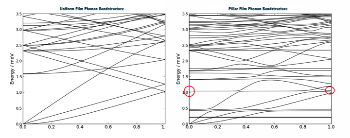
The vibrational modes illustrated below are calculated for the localized state marked in the bandstructure plot above at Γ and X points, respectively. The displacements are enhanced for a clearer view. This is controlled by the Temperature setting in the Vibration Visualizer plugin.

References