Magnetic Anisotropy Energy of Fe-MgO-Fe MTJ structure

Version: S-2021.06

Downloads & Links

PDF version
Fe21-MgO7-relaxed.py
orbital-moment-script.py
MagneticAnisotropyEnergy
Basic QuantumATK Tutorial
ATK Reference Manual

In this tutorial you will learn how to use the MagneticAnisotropyEnergy study object to calculate the perpendicular magnetic anisotropy (PMA) energy of a Fe-MgO-Fe magnetic tunnel junction (MTJ) structure.

You will learn how to analyze site- and orbital projected magnetic anisotropy energy (MAE) values and compare the results to OrbitalMoment based calculations.

The MAE is of central interest for both fundamental and practical reasons, with STT-MRAM being one of the most important technological examples.

Note

This tutorial builds on the introductory MAE tutorial treating a bulk system: Bulk Magnetic Anisotropy Energy, and it is assumed that the reader is familiar with its contents. If you are not already familiar with MAE calculations in QuantumATK, we suggest you go through that tutorial before continuing here.

Introduction

One of the key requirements of an STT-MRAM device is to be able to store information. This requires a sufficiently high energy-barrier between the ‘1’ and ‘0’ states of the system, such that a switch does not happen due to random thermal fluctuations. The MAE is a key element in determining the energy barrier and thus the thermal stability of a STT-MRAM memory unit. The stability factor is given by [1]:

\[\Delta = \frac{H_K M_S V}{2k_B T}\]

where \(H_K\) is the anisotropy field, \(M_S\) is the saturation magnetization, \(V\) is the cell volume, \(k_B\) is the Boltzmann constant and \(T\) is the temperature.

When the magnetization direction is perpendicular to the interfaces of different materials, the cell design is called PP (perpendicular to plane) and is the design in focus for this tutorial [1].

For PP cells, \(H_K\) is determined by the PMA which has three main contributions: (i) contribution from the bulk of the magnetic material, bulk PMA, (ii) contribution from the interfaces and surfaces, interfacial PMA (iPMA), and (iii) from the shape anisotropy. Bulk Fe in the BCC phase has vanishing bulk PMA, while the iPMA can be substantial and is the focus of this tutorial.

In this tutorial we will calculate the PMA using the MagneticAnisotropyEnergy study object, which uses the force theorem to evaluate the energy difference between two magnetization directions. More information about the force theorem and validation of its use can be found in the reference manual: MagneticAnisotropyEnergy and in the tutorial: Bulk Magnetic Anisotropy Energy.

Fe-MgO-Fe MTJ structure

We begin by setting up the atomic structure of a Fe-MgO-Fe structure. Start by opening the Builder. In the Builder do the following (see image below):

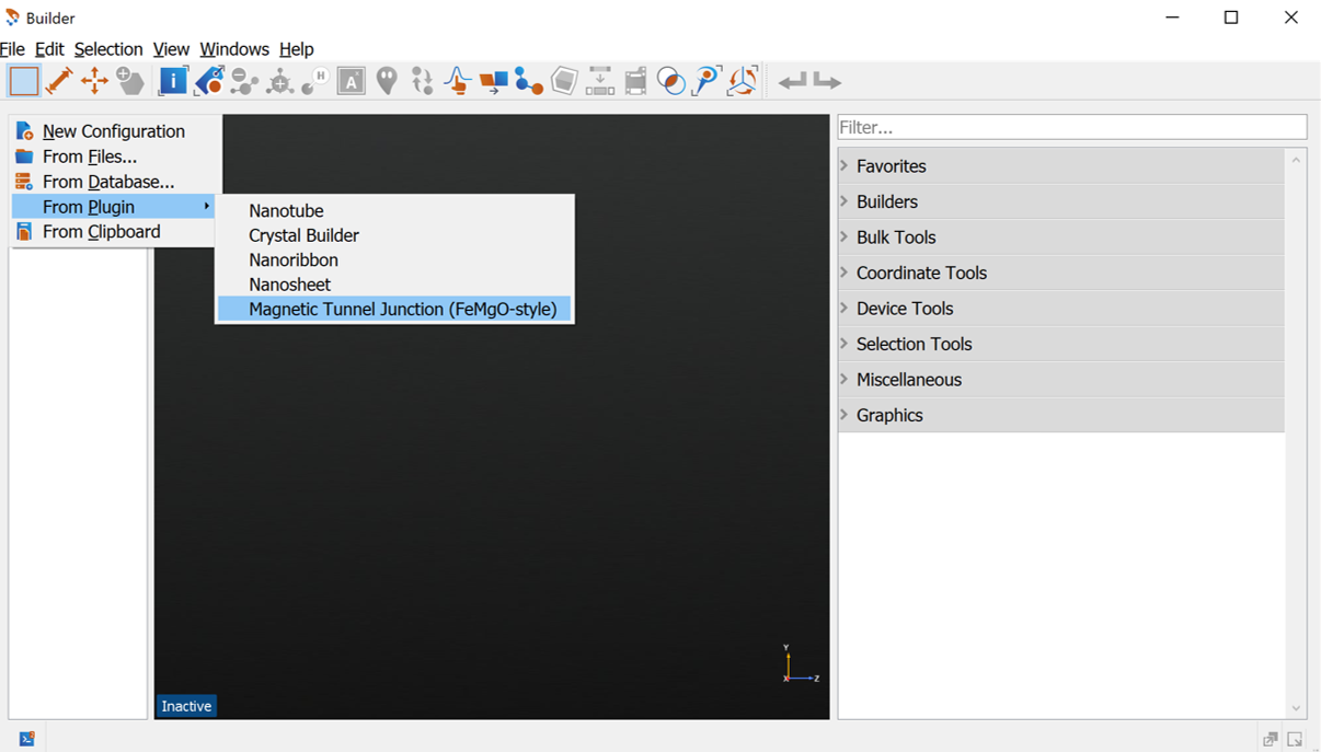
• Press the Add icon

• Select From Plugin

• Select Magnetic Tunnel Junction (FeMgO-style)

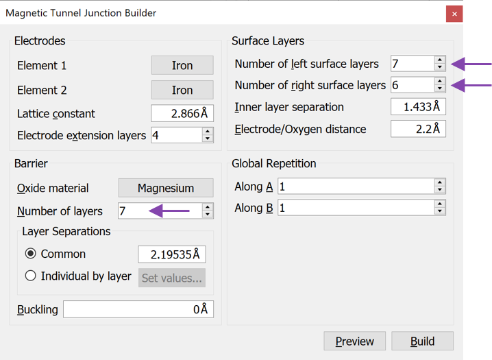
In the Magnetic Tunnel Junction Builder apply the following changes (see image below)

• For the Barrier set the Number of layers to 7

• For the Surface Layers:

  • Set Number of left surface layers to 7

  • Set Number of right surface layers to 6

• Press Build

You now have a DeviceConfiguration in the Builder. Split the device into electrodes and central region using the button indicated in the figure below.

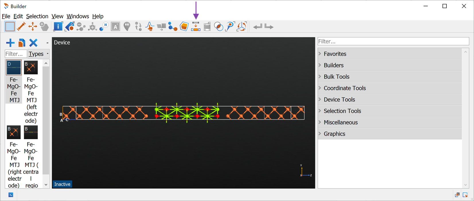
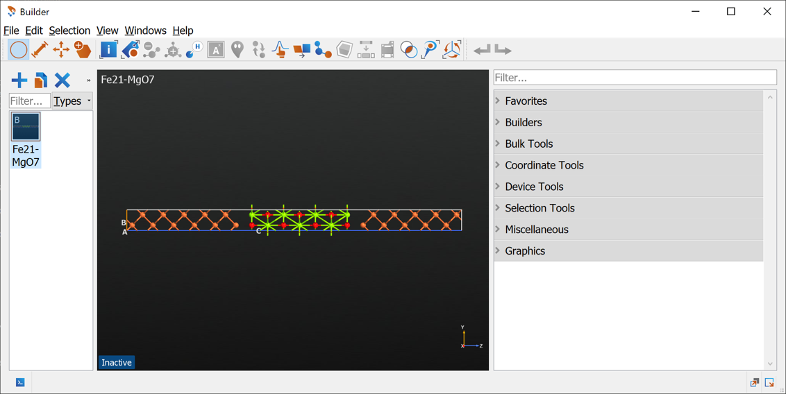
Once the device has been split, you can delete the original device structure as well as the electrodes. Finally rename the remaining central region to Fe21-MgO7 (press F2), indicating that the structure has 21 Fe layers and 7 MgO layers. Your builder should now look as below.

Note

The although we setup the MTJ structure with 6 and 7 surface layers, we ended up with a bulk configuration of 21 layers. The reason is that we have also included the 4 electrode extension layers on both sides. The total number of layers is thus the sum of left and right surface layers and the electrode extension layers, \(6+7+4+4=21\).

Send the structure to the Script Generator using the Send-to button.

Structural relaxation

The next step will be to relax the structure. In the Script Generator do the following:

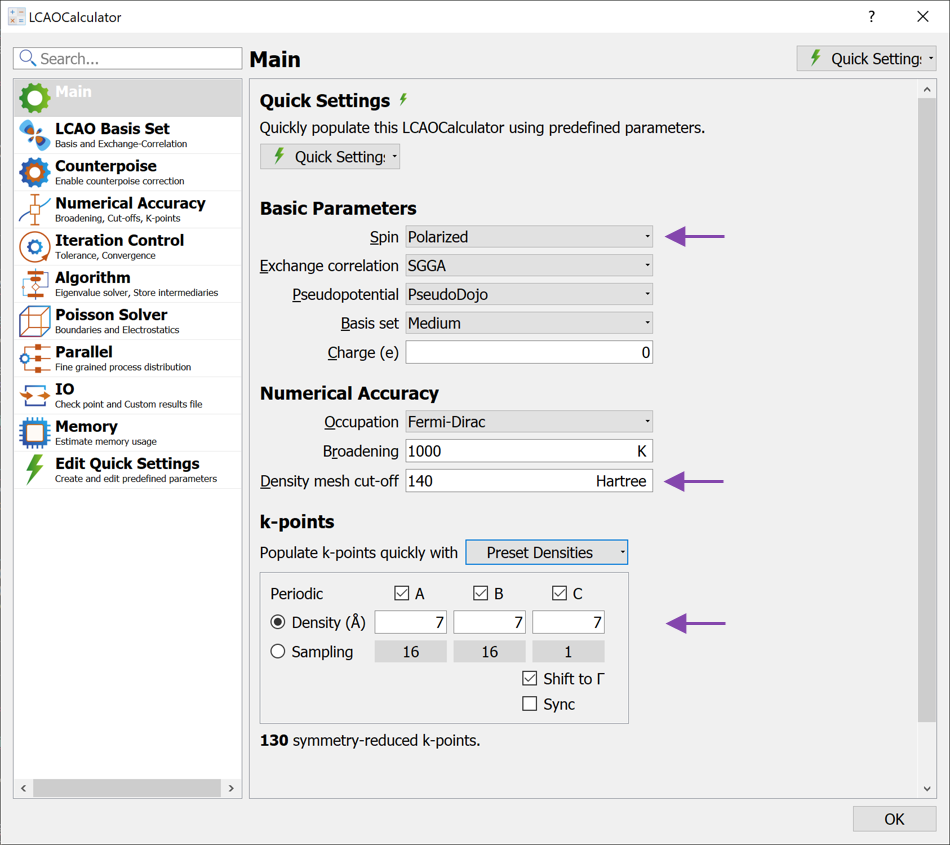
• Add an LCAOCalculator block and open it (see image below):

  • Change the Spin to Polarized. This is necessary since iron is magnetic and cannot be correctly modeled with an unpolarized calculation.

  • Increase the Density mesh cut-off to 140 Hartree. For this configuration, the geometry optimization converges faster with this increase.

  • Increase the k-point density to 7 Å (select from the Preset Densities combo box).

  • Leave the remaining settings as defaults and close the widget again.

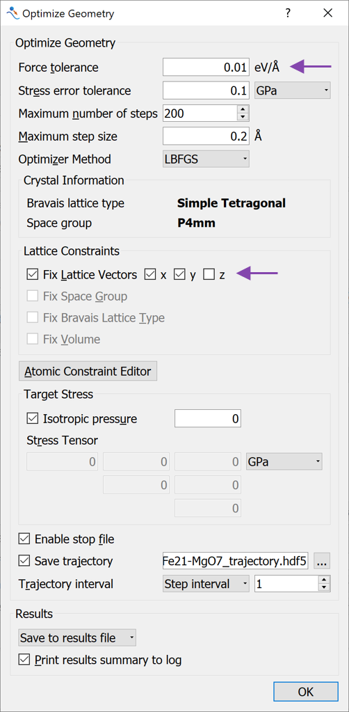
• Add an OptimizeGeometry block to the script and open it to apply the following changes (see image below):

  • Change the Force tolerance to 0.01 eV/Å

  • Uncheck the Fix Lattice Vectors for the z direction. This allows the C-lattice vector in the unit cell to be optimized. The A- and B- lattice vectors are kept fixed, although the atoms are allowed to move also in the x- and y-directions.

You are now ready to submit the calculations. Send the calculation to the Job Manager using the Send-to button and run the calculation. The calculation can take several hours to complete even when run with multiple MPI processes. For this reason we provide here the relaxed structure: Fe21-MgO7-relaxed.py. Either wait for the Geometry Optimization job to finish or download the relaxed configuration to obtain the relaxed configuration. Transfer the relaxed configuration to the Script Generator.

MagneticAnisotropyEnergy calculation

In the Script Generator do the following:

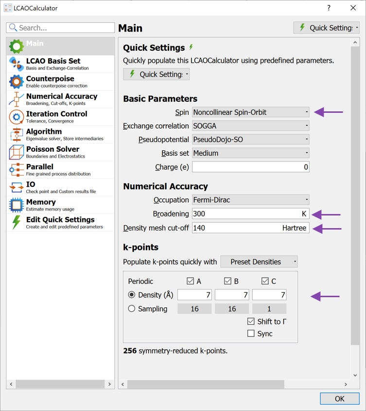
• Add an LCAOCalculator and open it (see image below):

  • Change the Spin to Noncollinear Spin-Orbit.

  • Set the Broadening to 300 K

  • Increase the Density mesh cut-off to 140 Hartree.

  • Increase the k-point density to 7 Å (select from the Preset Densities combo box).

  • Leave the remaining settings as defaults and close the widget again.

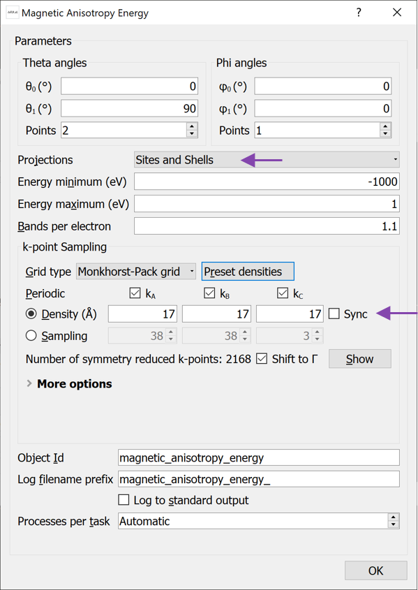
• Add a MagneticAnisotropyEnergy study object and open it (see image below):

  • Change Projections to Sites and Shells. This will calculate the contribution to the MAE from the s, p, d and f shells on each atom.

  • Increase the k-point density to 17 Å (choose this value from the Preset densities).

  • Leave the remaining settings as defaults and close the widget again.

Note

The total MAE will always be calculated irrespective of which Projections have been selected. The choice of Projections only determines which kind of analysis can be performed. The default choice of Sites allows a decomposition of the MAE onto atomic sites, but no information about which orbitals are involved. Choosing Sites and Shells gives additional information about which shells (s, p, d, f) contribute, while choosing Sites and Orbitals give detailed information about individual orbitals, e.g. \(p_x,\; p_y,\; p_z\) etc.

If more detailed projections are chosen, more memory will be required and the calculation time will also increase.

If you are only interested in the total MAE value, it can be beneficial to choose No Projection as this will lower the required memory and reduce the computation time.

Send the calculation to the Job Manager using the Send-to button and run the calculation. The calculation can take several hours. On a single node with 24 cores, the calculation takes about two hours.

Analyzing the results

Once the calculation has finished we are ready to analyze the results:

• Check the hdf5 file on the LabFloor.

• Mark the MagneticAnisotropyEnergy object and open the analyzer Magnetic Anisotropy Energy…

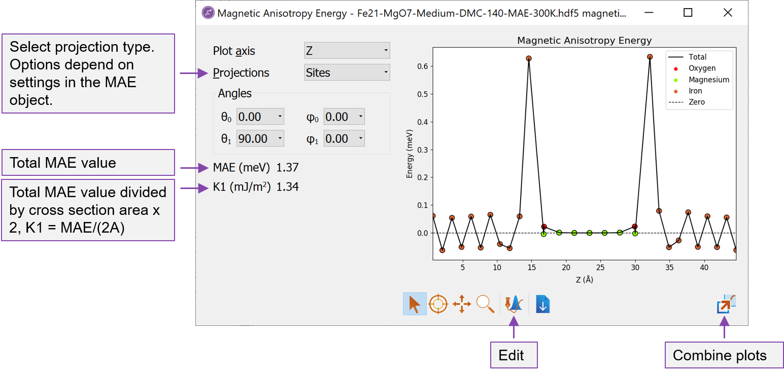
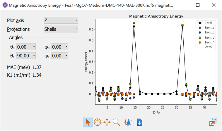
Fig. 15 The Magnetic Anisotropy Energy analyzer shows both the total MAE and the projected values.

The Magnetic Anisotropy Energy analyzer opens with a window showing the site-resolved contributions to the MAE (if No Projection was chosen when setting up the MAE object, this plot will be empty). The type of projections can be selected to the left of the plot.

In the lower left, the total MAE is shown in units of meV. Just below is shown the K1 value, which here is defined as \(K1 = MAE/(2\cdot A)\) where \(A\) is the cross section area. The factor \(1/2\) accounts for the fact that most systems will have two equivalent interfaces. If this is not the case, the K1 value needs to be determined manually.

From the analyzer, we see that:

• The MAE value is positive showing that the perpendicular (out-of-plane) magnetization is the energetically most favorable and the Fe-MgO-Fe structure is thus suitable for a PP cell design (note however, that the shape anisotropy, which favors in-plane magnetization, is not taken into account).

• The contribution to the positive MAE mainly comes from the interface Fe layers.

• The bulk Fe layers furthest away from the Fe-MgO interface have a smaller contribution to the MAE and shows an oscillating behaviour, summing up to a very small contribution. This means that K1 equals the surface anisotropy energy density, \(\sigma\).

• The Mg and O atoms essentially do not contribute to the MAE.

Since the MagneticAnisotropyEnergy object was calculated with Projections set to Sites and Shells we also have the possibility to analyze which orbital shells are responsible for the MAE:

• Change Projections to Shells in the MAE analyzer window.

Several new lines are now added to the plot and at first sight it appears difficult to analyze. However, in QuantumATK it is very easy to customize plots. Since the Mg and O atoms are unimportant for the total MAE, we do not want to show results for those. In order to edit the plot do the following:

• Press the Edit button (see image above) or simply press e.

• Mark all the Oxygen and Magnesium lines

• Un-check the Visible box (see image below)

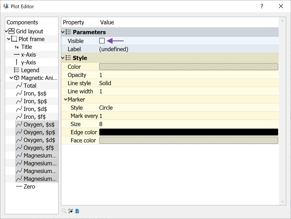
• Now mark all the Iron lines

• Change the Line style to No line (see image below)

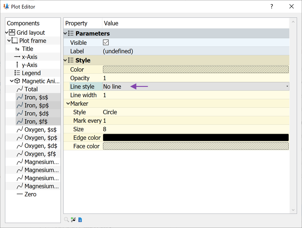
We have now removed all the oxygen and magnesium data from the plot, as well as the lines between the points for the iron atoms. Now the analyzer should look like the image below.

It is now evident that the finite MAE value essentially only comes from the Fe d-orbitals. Such information can indeed be very useful since it provides insight into how the MAE can be optimized by modifying the Fe d-orbitals.

Tip

Such analysis and experiments have been the focus of the Horizon 2020 COSMICS project.

Orbital moment analysis

We learned from the analysis above that the MAE in the Fe-MgO-Fe MTJ structure essentially comes from the Fe d-orbitals. Due to this simple contribution and since the spin-orbit coupling in iron is rather weak, it is possible to estimate the MAE with a more perturbative approach using the Bruno formula [2]:

\[MAE = -\frac{\xi_{Fe-d}}{4} ( L_x - L_z )\]

Here \(L_x\) is the x-component of the orbital moment, when the spin orientation is along the x-axis (\(\theta=90^\circ\)) and \(L_z\) is the z-component of the orbital moment, when the spin orientation is along the z-axis (\(\theta=0^\circ\)). \(\xi_{Fe-d}\) is the spin-orbit coupling strength from the Fe d-orbitals.

The orbital moment can be calculated in QuantumATK, for systems with Spin set to Noncollinear Spin-Orbit. Usually a non-selfconsistent spin-orbit calculation restarting from the polarized one is sufficient.

Since we already have non-selfconsistently updated spin-orbit calculations from the MagneticAnisotropyEnergy we can use these for an OrbitalMoment analysis. In the script, where the MagneticAnisotropyEnergy was calculated, we can insert the following lines at the end of the script:

# Get the non-selfconsistently updated spin-orbit configurations for the specified
# (theta, phi) angles.
configuration_so_0 = magnetic_anisotropy_energy.updatedSpinOrbitConfiguration(0*Degrees, 0*Degrees)
configuration_so_90 = magnetic_anisotropy_energy.updatedSpinOrbitConfiguration(90*Degrees, 0*Degrees)

# -------------------------------------------------------------
# Orbital Moment
# -------------------------------------------------------------
kpoints = KpointDensity(
    density_a=7.0*Angstrom,
    force_timereversal=False,
    )

orbital_moment = OrbitalMoment(
    configuration=configuration_so_0,
    kpoints=kpoints,
    temperature=300.0*Kelvin,
)
nlsave('Fe21-MgO7.hdf5', orbital_moment, object_id='Orbital moment 0')

orbital_moment = OrbitalMoment(
    configuration=configuration_so_90,
    kpoints=kpoints,
    temperature=300.0*Kelvin,
)
nlsave('Fe21-MgO7.hdf5', orbital_moment, object_id='Orbital moment 90')

Note

The MagneticAnisotropyEnergy is a study object, which has a number of task to complete, when called with magnetic_anisotropy_energy.update(). The study upject keeps track on which tasks have already been finished and will not do them again. Therefore, when the lines above to your script with the MagneticAnisotropyEnergy calculation, the MAE calculation will not do any work (except for detecting that it has already finished all the tasks), and the script will quickly proceed to the last part.

The orbital moment can also be setup using the Script Generator. In this case, it is important to remember that the analysis of orbital moment using the Bruno formula requires two calculations for different spin orientations. Such a script is provided here, where a self-consistent polarized calculation is followed by two non-selfconsistent spin orbit calculation for two different initial spin orientations: orbital-moment-script.py.

Once the orbital moments have been calculated, the results can be analyzed with the following script.

import pylab

# File name.
filename = 'Fe21-MgO7.hdf5'

orbital_moment_z = nlread(filename, object_id='Orbital moment 0')[0]
orbital_moment_x = nlread(filename, object_id='Orbital moment 90')[0]

# Spin-orbit coupling strength
e_so = 60 * meV

# Get the total moment
L_z = orbital_moment_z.orbitalMoment()[2] / bohr_magneton
L_x = orbital_moment_x.orbitalMoment()[0] / bohr_magneton

# Calculate the MAE using Bruno's formula
mae = -e_so / 4 * (L_x - L_z)

nlprint('Total MAE (Bruno formula) = {: .2f} meV'.format(mae.inUnitsOf(meV)))


# Get the atom resolved moments
L_z_atom = orbital_moment_z.atomResolvedOrbitalMoment()[:, 2] / bohr_magneton
L_x_atom = orbital_moment_x.atomResolvedOrbitalMoment()[:, 0] / bohr_magneton

mae_atom = -e_so / 4 * (L_x_atom - L_z_atom)

# Get the z-coordinates
z = orbital_moment_z._configuration().cartesianCoordinates()[:, 2].inUnitsOf(Ang)

pylab.figure()
pylab.plot(z, mae_atom, 'ko-')
pylab.xlabel('z ($\\AA$)')
pylab.ylabel('MAE (meV)')
pylab.show()

Note

In the analysis we use that the spin-orbit coupling energy of the Fe d-orbitals is 60 meV [3].

The outcome of the script is that the total PMA obtained from the Bruno formula is

Total MAE (Bruno formula) =  1.16 meV

The total MAE (PMA) is thus in fairly good agreement with the Force theorem (FT) result obtained from the MagneticAnisotropyEnergy object of 1.37 meV. It is also possible to get an atom-resolved plot as shown below, which is also produced by the same script:

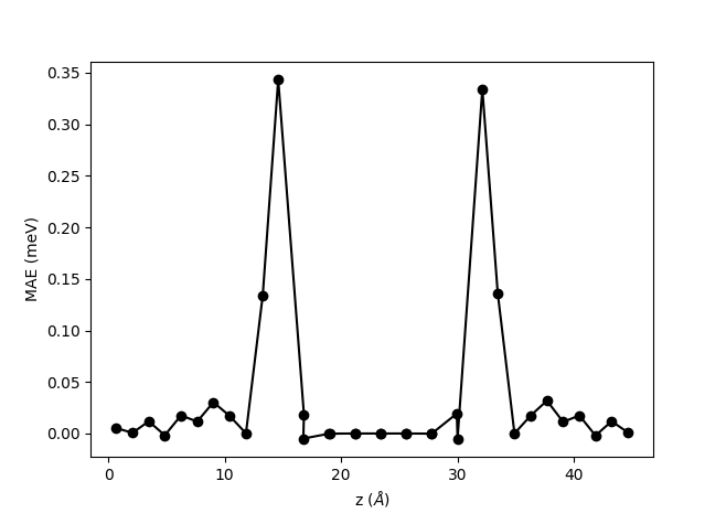
The atom-resolved MAE obtained from the Bruno formula clearly shows a similar behavior as the site-resolved MAE plot shown above: The main contribution comes from the interface Fe layers, while the bulk Fe has a vanishing contribution. However, there are some quantitative differences. The results obtained from the orbital moment and the Bruno formula show a rather large contribution from the second interface layer, which is not evident in the FT results. The oscillations in the bulk part of the Fe also comes out slightly smaller from the Bruno formula than from the FT.

The fairly good agreement between the Bruno formula and the FT method serves to validate both approaches. It should, however, be noticed that such a good agreement is not always the case. In calculations including heavier elements with stronger spin orbit coupling, it has been shown that the Bruno formula does not agree with the FT method [4] or self-consistent total energy calculations. The Bruno formula should therefore be used with care, while the FT method used in the MagneticAnosotropyEnergy object is in good agreement with total energy calculations, also for heavy elements [4]. For more details about comparing the FT method with total energies see the tutorial Bulk Magnetic Anisotropy Energy.

What causes the PMA?

In the above sections we have seen that the contribution to the interfacial PMA comes mainly from the interface Fe layers, while bulk Fe has much smaller contribution. But what causes the positive interfacial PMA? There can be (at least) three sources:

1. Fe-O hybridization. The Fe d-orbitals hybridizes with the O orbitals. In previous studies it has e.g. been shown theoretically and experimentally that hybridization with graphene or C60 increases the PMA of Co surfaces.

2. Strain and relaxation effects. The atomic positions are slightly distorted close to the surface compared to the bulk coordinates.

3. Interface asymmetry. This asymmetry exist at any interface, also at a Fe surface, i.e. a Fe - vacuum interface.

In this section we will try to analyze and quantify the contribution from each of the three sources. Since the calculations are performed in the same way as above, we will focus on the results and analysis. We will do that by comparing the total and projected MAE for different configurations as detailed below.

We will start by analyzing the relative importance of the Fe-O hybridization vs. the interface asymmetry. For doing this, we remove the MgO layers from the relaxed Fe-MgO-Fe configuration, and calculate the MagneticAnisotropyEnergy for this 21 layer Fe slab. Since we do not want to mix in contributions from strain effects, we keep the Fe atoms in the same positions and do not perform any further relaxations. The calculation can be run with this script Fe21-vacuum.py.

In order to address the effect of strain effects, we also repeat the MagneticAnisotropyEnergy calculation for the unrelaxed configuration produced directly by the MTJ builder plugin. The calculation can be run with this script Fe21-MgO7-unrelaxed.py.

The total PMA calculated for the three systems is shown in the table below. The total PMA is largest for the relaxed Fe-MgO-Fe structure.

Structure
Fe-MgO-Fe Relaxed	Fe-MgO-Fe Unrelaxed	Fe-vacuum
1.37 meV	0.68 meV	0.79 meV

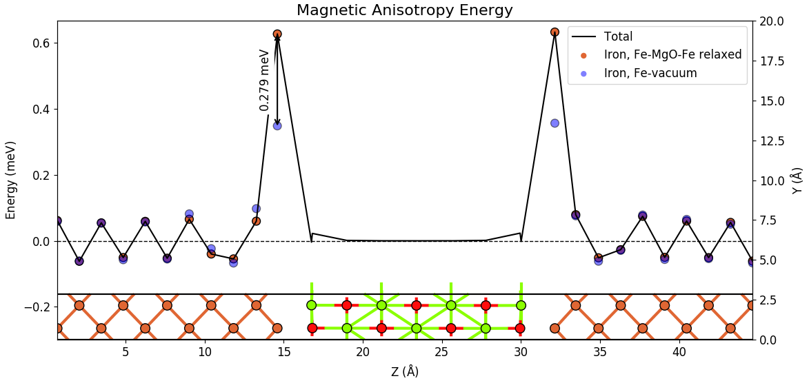
The figure below compare the relaxed Fe-MgO-Fe structure with the Fe-vacuum structure, where the Fe atoms are in the same positions. We observe that the interface Fe layes have a higher PMA value when hybridizing with the oxygen atoms in the Fe-MgO-Fe structure than when interfacing vacuum in the Fe-vacuum system. For each interface Fe atom the PMA is increased by 0.28 meV. The Fe-O hybridization thus have a significant influence increasing the total PMA from 0.79 meV for the Fe-vacuum structure to 1.37 meV for the Fe-MgO-Fe structure. It is interesting to see that the Fe-O hybridization is a very local effect essentially only affecting the PMA value of the interface Fe layers, while all the other Fe atoms essentially have the same PMA value in the Fe-MgO-Fe and Fe-vacuum structures.

The interface asymmetry, which is present in both the Fe-MgO-Fe structure and the Fe-vacuum structure (although a different asymmetry) is also an important effect since the Fe-vacuum structure also has a reasonably high PMA value of 0.79 meV, whereas bulk Fe has close to zero PMA.

Tip

The figure above shows the structure of the configuration together with the MAE plot. This figure has been made with the following procedure:

• Open the Magnetic Anisotropy Energy analyzer for both the Fe-MgO-Fe and the Fe-vacuum structures and edit the plots individually.

• Combine the two plots by dragging one onto the other using the Combine plots button (see Fig. 15 above).

• Mark the Fe-MgO-Fe structure on the LabFloor and select the Configuration Plot from the right column of analyzers.

• Combine the Configuration plot with the MAE plots.

• Adjust y-axis limits to make the plot look as you want (use the edit button or press e - see Fig. 15 above)..

Next we address the effect of strain and relaxation effects. From the table above we see that the unrelaxed Fe-MgO-Fe structure has a total PMA value of 0.68 meV, i.e. only about half the value of the relaxed structure. This difference illustrates the importance of including the strain and relaxation effects and it also shows that PMA values are very sensitive to small details in the atomic structure.

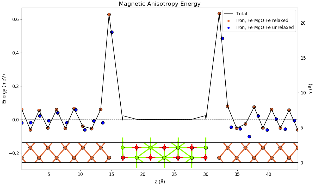
The above figure compares the atomic contributions to the PMA for relaxed and unrelaxed Fe-MgO-structure. The unrelaxed structure has smaller PMA values at the interface layers and shows smaller oscillations in the bulk part of the Fe. However, the qualitative picture of the PMA being determined by the interface layers, remain the same for the two configurations.

COSMICS project

The MagneticAnisotropyEnergy study object has been developed within the project COSMICS founded by the European Union’s Horizon 2020 research and innovation program under Grant Agreement No. 766726. Details about the object can be found on the manual page here MagneticAnisotropyEnergy. Application of the MagneticAnisotropyEnergy object to metallic slabs and comparison with QuantumEspresso and tight-binding calculations are presented in ref [5].

More information about the COSMICS project can be found here: http://cosmics-h2020.eu/

References

[1] (1,2)

A V Khvalkovskiy, D Apalkov, S Watts, R Chepulskii, R S Beach, A Ong, X Tang, A Driskill-Smith, W H Butler, P B Visscher, D Lottis, E Chen, V Nikitin, and M Krounbi. Basic principles of stt-mram cell operation in memory arrays. Journal of Physics D: Applied Physics, 46(7):074001, feb 2013. URL: https://doi.org/10.1088/0022-3727/46/7/074001, doi:10.1088/0022-3727/46/7/074001.

[2]

Patrick Bruno. Tight-binding approach to the orbital magnetic moment and magnetocrystalline anisotropy of transition-metal monolayers. Phys. Rev. B, 39:865–868, Jan 1989. URL: https://link.aps.org/doi/10.1103/PhysRevB.39.865, doi:10.1103/PhysRevB.39.865.

[3]

G. Autes, C. Barreteau, D. Spanjaard, and M. Desjonqueres. Magnetism of iron: from the bulk to the monatomic wire. Journal of Physics: Condensed Matter, 18(29):6785–6813, jul 2006. doi:10.1088/0953-8984/18/29/018.

[4] (1,2)

M. Blanco-Rey, J.I. Cerda, and A. Arnau. Validity of perturbative methods to treat the spin–orbit interaction: application to magnetocrystalline anisotropy. New J. Phys., 21:073054, 2019. URL: https://iopscience.iop.org/article/10.1088/1367-2630/ab3060.

[5]

L. Le Laurent, C. Barreteau, and T. Markussen. Magnetocrystalline anisotropy of fe, co, and ni slabs from density functional theory and tight-binding models. Phys. Rev. B, 100:174426, Nov 2019. URL: https://link.aps.org/doi/10.1103/PhysRevB.100.174426, doi:10.1103/PhysRevB.100.174426.