DFT-D and basis-set superposition error
In this tutorial you will calculate the distance between two graphene layers. To calculate this distance you will need to account properly for van der Waals interactions (also termed dispersion interactions). The latter are underestimated by local (LDA) and semi-local (GGA) exchange-correlation functionals. As a result, using these functionals the layers do not bind (or bind too weakly) and the minimal total energy configuration becomes one where the layers are infinitely separated. The long-range van der Waals interaction will be included through the semi-empirical corrections by Grimme D2 [1] and D3 [2]. These corrections do not attempt to describe the actual source of the interaction (fluctuating dipoles) but rather its effect on the DFT mean-field effective potential.
You will also learn that incompleteness of the LCAO basis set can give rise to a so-called basis set superposition error (BSSE). The BSSE will contribute with an artificial attraction between the graphene layers, which actually partly compensates for the lack of van der Waals attraction, so with some exchange-correlation potentials the graphene layers will bind, but for the wrong reason. Thus, if you introduce the Grimme correction but do not account for BSSE, the layers will instead bind too strongly and a too small layer separation will be obtained. To remove the BSSE you will use the counterpoise correction [3].
The BSSE is mostly noticeable when computing cohesive energies or binding energies where two subsystems can be clearly defined, like in the case of a molecule on a surface [4] or, as in this tutorial, in layered systems. It is however also an issue for vacancy formation energies, where the material surrounding the vacancy has a lower number of basis orbitals than available in the vacancy case [5].
The DFT-D dispersion corrections
The corrections by developed by Grimme an co-workers [1][2] add an additional term \({E}_\mathrm{disp}\) to the DFT total energy \({E}_\mathrm{DFT}\) in order to account for van der Waals interactions:
The D2 and D3 corrections differ in the way the term \({E}_\mathrm{disp}\) is evaluated.
D2 correction
In the D2 correction [1] the \({E}_\mathrm{disp}\) term include only two-body energies and is given by an attractive semi-empirical pair potential \(V^{\mathrm{PP}}\) which accounts only for the lowest-order dispersion term:
where \(R_A\) (\(R_B\)) and \(R_{AB}\) are the atomic number of atom \(A\) (atom \(B\)) and the interatomic distance, respectively. The global scaling parameter \(S_6\) has been fitted to reproduce the thermochemical properties of a large training set of molecules and depends on the exchange-correlation functional employed.
The pair potential between two atoms with atomic numbers A and B separated by a distance \(R_{AB}\) is:
where
is a damping function and \(C_6\) and \(R_0\) are element-specific parameters. Typically, the damping factor \(d_6\) is set to 20.
D3 correction
In the D3 correction [2], the \({E}_\mathrm{disp}\) term includes both two- and three-body energies:
Two-body energy term
The two-body energy include dispersion terms up to the 8th order:
In the equation above, \(S_6 = 1\) for all elements, whereas \(S_8\) depends on the exchange-correlation functional employed. The 6th order pair potential is
where
and the 8th order pair potential is constructed using the 6th order data as:
\(C_{6, \mathrm{ref}}^{AB}\) are reference dispersion coefficients derived from time-dependent DFT (TDDFT) calculations using a training set of \(N_A\) (\(N_B\)) molecules for atom A (B). \(\langle r^2 \rangle\) and \(\langle r^4 \rangle\) are geometrically averaged multipole-type expectation values derived from atomic densities. \(n^A\) and \(n^A_i\) (\(n^B\) and \(n^B_j\)) are the atomic fractional coordination number for atom A in the system and in the \(i\)-th (\(j\)-th) molecule of training set \(N_A\) (\(N_B\)),
where \(R_{A,\mathrm{cov}}\) and \(R_{B,\mathrm{cov}}\) have been taken from [6]. Finally, the damping functions for 6th (\(f_6(R_{AB})\)) and 8th (\(f_6(R_{AB})\)) orders terms are, respectively:
and
with \(R_0^{AB}\) being the cutoff radius for the \(AB\) element pair, and \(d_{6}\) and \(d_{8}\) are damping factors depending on the exchange-correlation functional.
Note
As it is evident from the equations above, in the D3 method \(V_6^{\mathrm{PP}}\) and \(V_8^{\mathrm{PP}}\) depend not only on the interatomic distance but also on the chemical enviroment of each atom via the fractional coordination number. This is one of the major differences compared to the D2 method.
Three-body energy term
The additional three-body energy contribution is evaluated as:
where the three-body potential \(V^{\mathrm{TBP}}\) is constructed starting from the two-body terms,
using the following damping function,
where the geometrically averaged radii are
Note
The evaluation of \({E}^{(3)}\) changes the scaling behavior of the D3 algorithm from \(O(N^2)\) to \(O(N^3)\), where \(N\) is the number of atoms. Computing the three-body energy term can therefore be extremely expensive for large systems. Since the magnitude of the \({E}^{(3)}\) energy correction is much smaller than the two-body energy correction \({E}^{(2)}\), the former is switched-off by default in QuantumATK.
BSSE and the counterpoise correction
In polyatomic systems, the so-called basis set superposition error (BSSE) arises due to the localised nature of the LCAO basis set. To understand the origin of the BSSE, consider a system formed by two subunits A and B. For simplicity, consider each subunit to be a single atom. When A and B are far apart, they are described only by the basis orbitals centered at their respective atomic nuclei. However, when A couples to B the basis functions centered at A overlap with those centered at B. As a result, part of the basis orbitals centered at B are available to describe A. This gives rise to an artificial attraction between A and B.
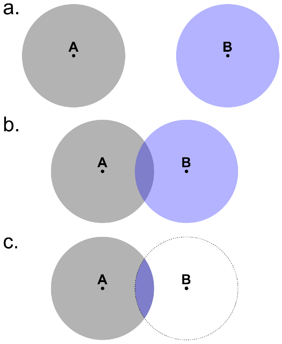
Fig. 125 Origin of the basis set superposition error. (a) A and B far apart from each other; (b) basis orbitals overlap when A couples to B; (c) the region in blue indicated the part of the basis orbitals centered at B that are available to describe A.
The BSSE can be minimized by using the counterpoise (CP) correction [3]:
where \(E_{AB}\) is the total energy of system AB and \(E\) is the counterpoise energy correction.
The counterpoise correction is obtained through:
where \(E_{A\tilde{B}}\) is the energy of system A in the AB basis, which is obtained by taking the full system at its equilibrium geometry and defining the atoms of B as ghost atoms.
Note
Ghost atoms have no charge and no mass, but they have basis orbitals, defined by whichever element (and basis set) that defines the atom if it was not a ghost.
The counterpoise correction is readily extended to several subunits, \(A_i\) , through:
where \(C_i\) is the \(A_i\) complement, i.e. the atoms not in region \(A_i\).
In the following section you will explicitly see the effects of these two corrections on the calculated equilibrium distance between two graphene layers.
Set-up the graphene bilayer system
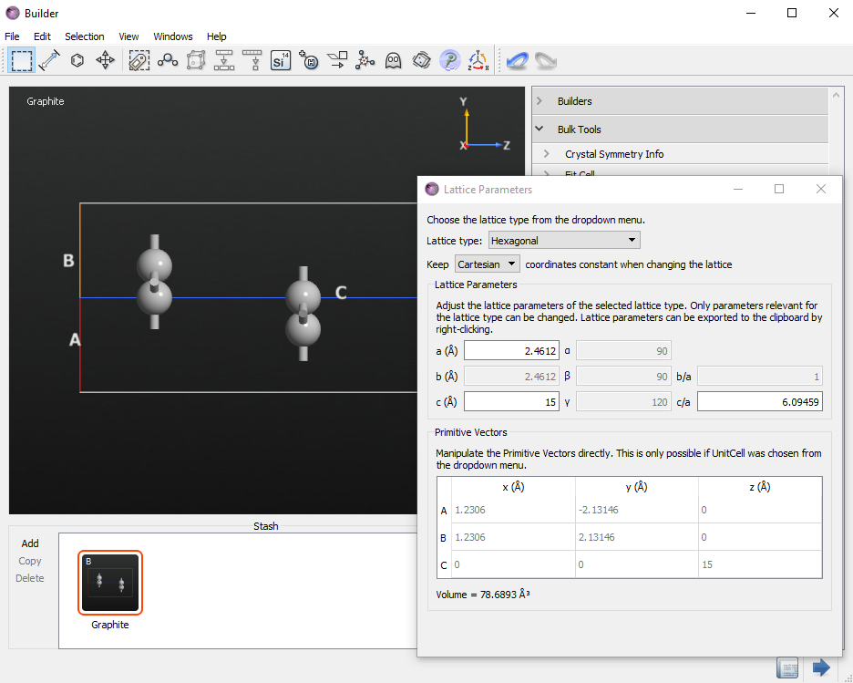
In the  Builder, click on , search for “Graphite” and add the structure to the stash.

Rename the structure as “graphene2”, then open and set the length of the C-vector to 15 Å. This transforms the graphite crystal into a bilayer graphene model.
Finally, center the geometry by using .
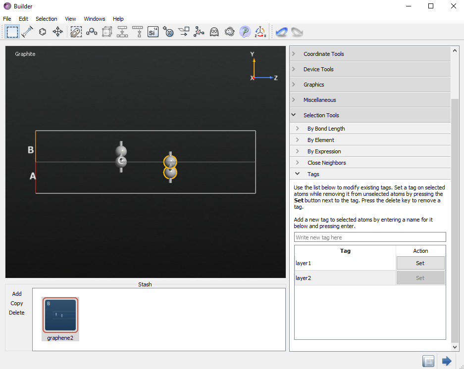
To finish the setup of the structure you must add a tag to each graphene layer. Tags are used to distinguish the two layers, in order to define the counterpoise correction. In order to add the tags, select the two atoms in the first graphene layer, open , write “layer1” in the bottommost field and press enter. Then, repeat the same steps for the second layer and tag it as
“layer2”.
Tip
You can check that the tags are correctly set using the Selection by Tag tool on the toolbar on the top of the Builder.
Geometry optimization without counterpoise correction
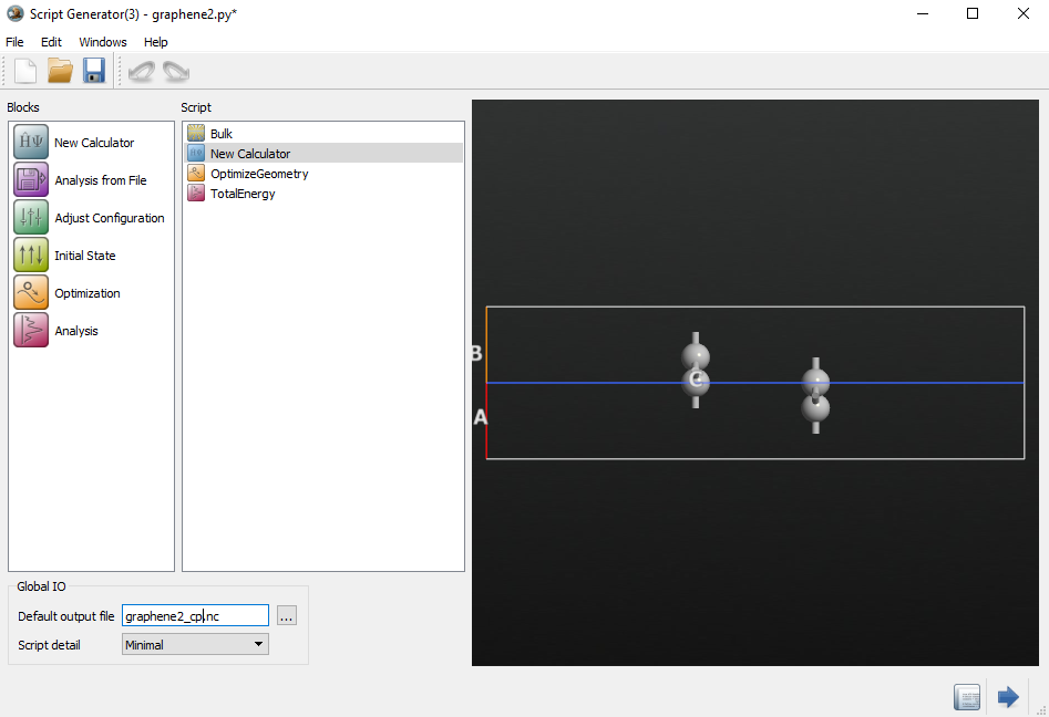
In the Builder, use the  button to send the graphene bilayer structure to the
  Script Generator. Change the default output name to “graphene2.nc” and add the following blocks:
Click on the  block and modify the following parameters:
Select the PBE functinal
Set the k-point sampling to a grid of \(11 \times 11 \times 1\) k-points.
Then, click on the  block and set the force tolerance to 0.01 eV/Å.

To start the calculation, click the Send To icon located in the lower-right of the scripter and select  Job Manager from the pop-up menu. Save the script as
 graphene2.py in the project directory.
The Job Manager will now pop up. Select the dropped script and press  icon to start the job.
Analysis of the optimized structure
To inspect the relaxed configuration, expand graphene on the LabFloor. The file contains two configurations gID000 and gID001. These are the input and relaxed structures, respectively.
Drag and drop the relaxed structure (gID001) to the Builder.
In the Builder, click the measurements option for distance, and measure the distance between the two carbon atoms that sit on top of each other in the Z direction. The interatomic distance is 3.47 Å, which is fairly close to the experimental value 3.32 Å [7]. As you will soon see, this is however a result of a cancellation of two errors!
Note
Most literature experimental values for the graphene interlayer distance are valid for graphite but not for the bilayer graphene system discussed in this tutorial. Hence there can be small differences between the calculated results and experimental data.

Including the counterpoise correction
You will now relax the geometry using the CP correction to correct for the basis set superposition error. To this end, open again the Scripter window where you set up the previous calculation.
Tip
All active tools are available through the Windows menu at the top of each tool.
Change the name of the output file to graphene2_cp.nc.
It is currently not possible to set up the CP correction in the Scripter. The CP correction must therefore be manually added by editing the QuantumATK script. Therefore, transfer the script to the  Editor using the Send To icon.
In the Editor, change the definition of the Calculator as follows:
#calculator = LCAOCalculator(
#    basis_set=basis_set,
#    exchange_correlation=exchange_correlation,
#    numerical_accuracy_parameters=numerical_accuracy_parameters,
#    correction_extension=correction_extension,
#    )

#BSSE CP correction
bsse_calculator = counterpoiseCorrected(LCAOCalculator, ["layer1", "layer2"])
calculator = bsse_calculator(
    basis_set=basis_set,
    exchange_correlation=exchange_correlation,
    numerical_accuracy_parameters=numerical_accuracy_parameters,
    correction_extension=correction_extension,
    )
Note how the system is separated into two parts (”layer1” and “layer2”) using the tags. The system can be divided into an arbitrary number of parts, and the counterpoise correction is applied to each couple of parts. The only requirement is that the parts are adjoint and sum up to the entire system.
Save the script as graphene2_cp.py, send it to the Job Manager and start the calculation. The run time will be 2–5 times longer than before, since now at each geometry optimization step, 5 different systems need to be calculated, viz. \(AB, A, A\tilde{B}, B, \tilde{A}B\).
When the calculation is done, inspect the interlayer distance and you will find it to be 4.23 Å. This is considerably larger than the previous result, and far from the experimental value (3.32 Å). As mentioned in the introduction, the BSSE creates an artificial attraction between the graphene layers, which reduces the interlayer distance. The counterpoise correction eliminates this error, but you are now left with the problem that the layers are essentially unbound, due to the omission of van der Waals forces.
Including the D2 dispersion correction
Since the interlayer distance calculated with the CP correction is too large, there must be a missing attractive contribution to the total force. This is the van der Waals (dispersion) force which is not correctly described with the PBE functional. The vdW contribution to the total forces can be approximately added using the semi-empirical DFT-D2 approach.
To add the D2 correction, drag and drop the graphene2_cp.nc file to the Scripter :
Change the output file to
graphene2_cp_d2.nc.Double-click
Double-click
Analysis and select TotalEnergy.
Now double-click the New Calculator block in the Script panel to open the calculator widget.
Under “Calculator setting” and “Basis set/Exchange correlation” select the Grimme DFT-D2 van der Waals correction. Note that you can modify all the specific parameters by clicking the Parameters button.

Double-click on the OptimizeGeometry block and set the force tolerance to 0.01 eV/Å.
Send the script to the Editor and edit the python script in order to add the counterpoise correction as you did before.
#----------------------------------------
# Grimme DFTD2
#----------------------------------------
correction_extension = GrimmeDFTD2(
    global_scale_factor=0.75,
    damping_factor=20.0,
    maximum_neighbour_distance=30.0*Ang,
    element_parameters={
        Carbon: [1.452*Ang, 1.75*J*nm**6/mol],
        },
    )

#BSSE CP correction
bsse_calculator = counterpoiseCorrected(LCAOCalculator, ["layer1", "layer2"])
calculator = bsse_calculator(
    basis_set=basis_set,
    exchange_correlation=exchange_correlation,
    numerical_accuracy_parameters=numerical_accuracy_parameters,
    correction_extension=correction_extension,
    )
Press the  save button and save the script as
 graphene2_cp_d2.py in the project directory.
Run the script and when the calculation is done, inspect the interlayer distance. You will now find it to be 3.31 Å. Thus, including the dispersion correction and accounting for BSSE, an interlayer distance close to the experimental result can be obtained.
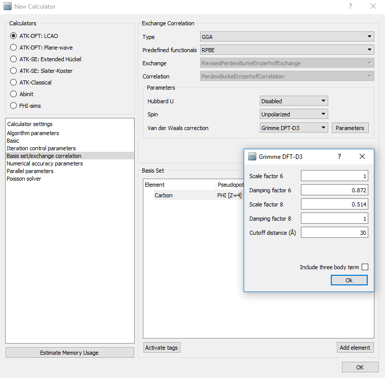
Including the D3 dispersion correction
The D3 correction can be applied in a similar way as shown for the D2 correction. However, as discussed in [2] in this case the best results for the interlayer distance and binding energy are obtained using a revised PBE-type functional (revPBE) instead of the original PBE. Therefore, when adding the D3 correction, one also need to change the exchange-correlation functional from PBE to revPBE as shown below (“RPBE” in the list of predefined functionals).
As discussed in the method section the D3 correction can be supplemented with a three-body energy term \({E}^{(3)}\) for an even more accurate evaluation of the vdW forces. However, evaluation of this term is computationally demanding, and the \({E}^{(3)}\) term is therefore not computed by default. If one wants to used DFT-D3 including three-body interactions, we suggest to first optimize the structure using DFT-D3 without the \({E}^{(3)}\) term, and then perfom a single-point calculation on the optimized geometry including the \({E}^{(3)}\) term.
Summary of the results
The result of the calculations are summarized in the following table.
EB (meV/atom) |
d (Å) |
|
PBE |
-15 |
3.47 |
PBE+CP |
-0.6 |
4.23 |
PBE-D2+CP |
-22.9 |
3.31 |
revPBE-D3+CP |
-22.6 |
3.35 |
revPBE-D3+CP+3body |
-18.6 |
3.36 |
The binding energy \(\Delta E\) of the bilayer system was calculated as:
where \(E_\mathrm{tot}^\mathrm{bilayer}\) and \(E_\mathrm{tot}^\mathrm{monolayer}\) are the total energies of bilayer and monolayer graphene respectively.
Note
The calculation of the binding energies must be consistent in terms of exchange-correlation functional and dispersion correction. For example, to obtain the PBE-D2+CP result, the single layer graphene reference calculation must be performed using DFT-D2.