Linear response current – how to compute it, and why it is often not a good idea
Version: 2016.2
In this tutorial, you will learn a simple way to calculate the linear response current and how it is different from the self-consistent result, the latter of which is necessary to exhibit negative differential resistance (NDR).
The question sometimes arises, why it is necessary to compute the I-V curve using finite-bias NEGF calculations – can’t one just use the zero-bias transmission spectrum (which is much cheaper to compute) and calculate the finite-bias current from that? This is indeed possible, but the result – the linear response current – is in most cases radically different from the current evaulated from a finite-bias self-consistent solution. The reason is fairly simple: The transmission spectrum is bias-dependent.
Important
In the linear response case, it is not possible to obtain negative differential resistance, since the current can only increase as the bias window opens up and you integrate an increasingly large part of the transmission spectrum. NDR is an important effect for applications, and is observed in a wide range of cases, but can only be obtained using a self-consistent finite-bias NEGF calculation.
Here well will demonstrate with a relatively simple example how to obtain the linear response current, and how it is different from the self-consistent result. The inspiration is taken from a recent work performed with QuantumATK by Yipeng An et al. [1]; in the article the authors used DFT, but we will consider the same system (specifically, the GE1 geometry) using a simple Slater-Koster tight-binding \(\pi\)-model.

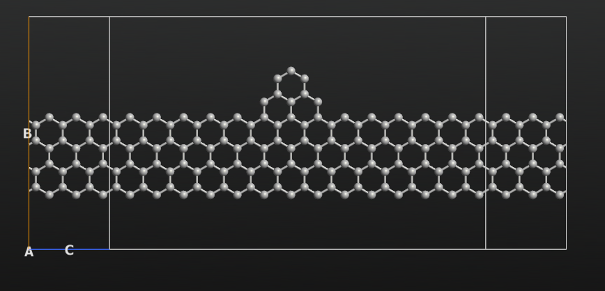
The geometry is shown below. We will not go into the details of how to create it;
it’s farily easy, using the  Builder: Create a large graphene
sheet and remove the atoms you don’t need. Note that for the Slater-Koster model
we don’t use any terminating hydrogen atoms.
Builder: Create a large graphene
sheet and remove the atoms you don’t need. Note that for the Slater-Koster model
we don’t use any terminating hydrogen atoms.
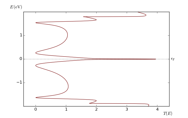
We can now compute the zero-bias transmission spectrum of this device. Use a
pre-made QuantumATK Python script for this: zero_bias.py. The script takes less than a minute
to run, even if there are 120 atoms in the central region. The resulting transmission
spectrum is shown below (select the Sum spin channel in the Curves drop-down
menu). The spectrum exhibits a pronounced peak at the Fermi level, which
is to be expected since the electrodes are zigzag graphene nanoribbons.
At this point, we can compute the linear response I-V curve by integrating the
transmission spectrum in an increasingly wide bias interval. QuantumATK supports this
calculation via a built-in method on the TransmissionSpectrum object.
Normally when you ask for the current,
current = transmission_spectrum.current()
it will be evaluated for the bias that was used when computing the transmission spectrum. However, it is also possible to specify another set of electrode voltages, which will then be used instead. Thus, if the transmission spectrum, as in our case, was computed for zero bias, you can use
current = transmission_spectrum.current(electrode_voltages=[-0.5,0.5]*Volt)
to get the linear response current at 1 V bias. You can therefore extract an entire linear response I-V curve by looping over a range of bias points and compute the linear response current at each bias.
Download the script linear_response.py and execute it. The script computes and plots
the linear response I-V curve. The result is shown below.
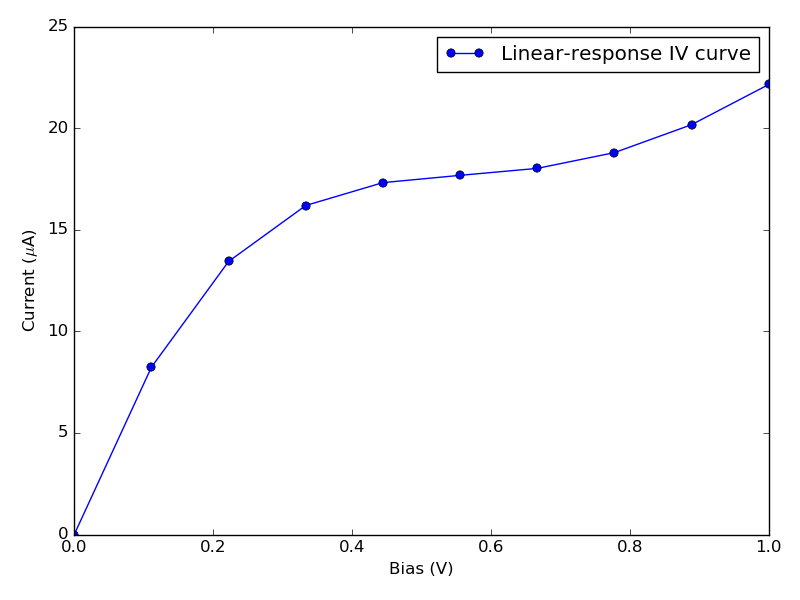
As expected, the current rises monotonically with the voltage – this is the only possible I-V curve that can be obtained this way, since we are integrating a non-negative function (the transmission spectrum) over an increasingly broad interval.
However, we know from [1] that this system exhibits negative
differential resistance, so something is not correct. Therefore, we will next
compute the self-consistent transmission spectrum for each bias.
Use this script: iv.py. It should take less than 5 minutes to run on a modern PC.
The script uses the IVcurve analysis object. From the QuantumATK LabFloor,
select the generated IVCurve item and click the IV-Plot plugin from the
right-hand plugins bar to visualize the results. Tick the boxes named
Additional plots and Spline interpolation.
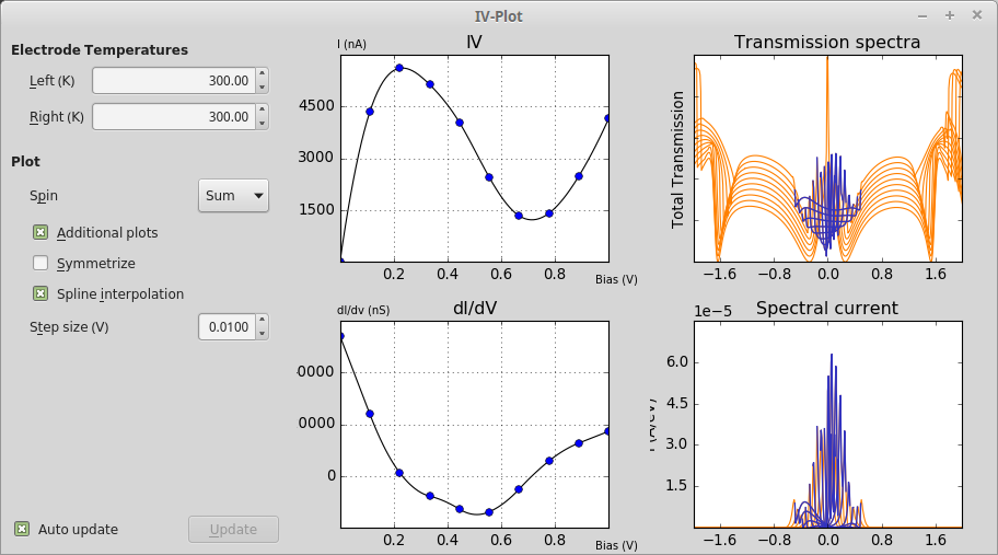
In this case we do indeed see NDR – the differential current is shown in the
lower-left plot, and it does become negative – and from the upper-right plot
of the transmission spectra
we can see why. The individual transmission spectra are strongly bias-dependent.
To illustrate this point even more clearly, we generate a contour plot of
the transmission spectra as a function of energy and bias, using a simple
script: transmission_contour.py.
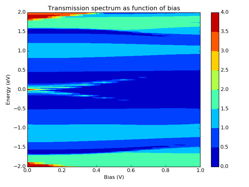
Clearly, the assumption of a bias-independent transmission spectrum is invalid in this system, and as mentioned above indeed in most device configurations.
References