Viscosity in liquids from molecular dynamics simulations
Version: P-2019.03
In this tutorial you will learn how to calculate the viscosity of different liquids using molecular dynamics (MD) simulations using the example of liquid methanol. Understanding viscosity is critical in designing a number of industrial chemical processes, as viscosity gives a description of how the liquid flows. This tutorial demonstrates how you can use the QuantumATK tools to simulate the viscosity of a simple fluid. This methodology can be applied to much more complicated fluids as well as mixtures.
To simulate the behavior of liquid methanol we use classical molecular dynamics to generate trajectories of the motion of molecules. These trajectories give the information necessary to statistically calculate the overall properties of the liquid. This tutorial also demonstrates how to set up and use specific bonded forcefields that have been created for these types of molecular problems.
Theory
Molecular viscosity
Viscosity is a measure of the friction between molecules passing each other in the fluid. There are a number of ways of estimating this friction[1], but one that is commonly used is the Einstein relationship where the viscosity \(\eta\) can be stated as[2]:
Here the quantities being integrated are the off-diagonal elements of the pressure tensor. The labels \(\alpha\) and \(\beta\) refer to these elements. The other quanities represented here are time \(t\), temperature \(T\), volume \(V\), and the Boltzmann constant \(k_B\).
An alternative method for calculating the viscosity is through the Green-Kubo relation[3]:
Here the quantity in the angle brackets is the autocorrelation function of the pressure tensor. As this auto-correlation function decays to zero at long timescales, the integral converges to give the fluid viscosity.
Both of these equations may produce similar results. For a trajectory with a large number of data points, the Green-Kubo expression can become computationally expensive. Calculating the autocorrelation function scales as \(O(N^2)\) where \(N\) is the number of data points. The Einstein relationship scales as only \(O(N)\). As calculating viscosity requires looking at a large number of data points, the focus will be placed on the Einstein relationship.
The pressure tensor itself is made up of contributions both from the motion of the atoms and also from how the atoms interact with the boundary conditions in the simulation. The pressure tensor can be given as:
Here \(m_i\) references the mass of atom \(i\), \(v_{i,\alpha}\) references the velocity of the atom \(i\) in the cartesian direction \(\alpha\) and \(E\) is the energy of the system which is being differentiated with respect to the strain \(\varepsilon_{\alpha\beta}\)
Force fields
Classical force fields work by replacing the computationally expensive calculation of electronic structure with simple functions designed to approximate the overall energy. This approach enables the effective simulation of much larger systems, well beyond what is possible with electronic structure calculations. One of the main challenges in this approach is fitting parameters for the replacement functions so they can accurately predict the energy.
One approach is to divide molecules up into a number of chemical types. Specific parameters can then be found for different types of interactions using these types. As an example, an sp3 carbon in ethane will have different associated potentials to an sp2 carbon in a benzene ring. As several combinations will be excluded based on how the types are defined, this limits the number of parameters that need to be found. Because parameters are fitted for specific atomic types and functions, these types of potentials can often be more accurate. As a trade-off these potentials are often more difficult to set up, as the chemical types for each atom need to be assigned for the structure. Potentials of this type also cannot model reactions, as the atom connectivity is needed to determine the chemical type.
In this tutorial you will use the OPLS-AA forcefield to model methanol[4]. The OPLS-AA forcefield uses atom types with specifically fitted potentials for those types. This tutorial covers how to set up calculations using these types of forcefields.
Computational procedure
Building the initial methanol configuration
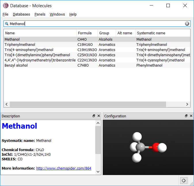
Open the Builder  and select .
Add the molecular structure of methanol from Database to the Stash, making
sure to choose the molecule database by selecting .
and select .
Add the molecular structure of methanol from Database to the Stash, making
sure to choose the molecule database by selecting .
Now the chemical types for each of the atoms needs to be assigned. OPLS methanol has 4 types:
‘CT’ for the tetrahedral carbon
‘HC’ for the hydrogens attached to the carbon
‘OH’ for the alcohol oxygen
‘HO’ for the alcohol hydrogen.
Select the three hydrogen atoms attached to the carbon. Set their types to ‘HC’ by going to and typing in the tag ‘HC’. You should now be able to select these atoms by using the tag. Repeat the process for the other three atom types.
Tip
When selecting atoms, holding down the Ctrl key adds atoms to the current selection, while holding down the Shift key removes them.
Next create a bulk model of liquid methanol by selecting . Drag the molecule of methanol from the stash into the molecule type column, and select 250 molecules. Set each cell length to 28 Ångstroms. Click Create.
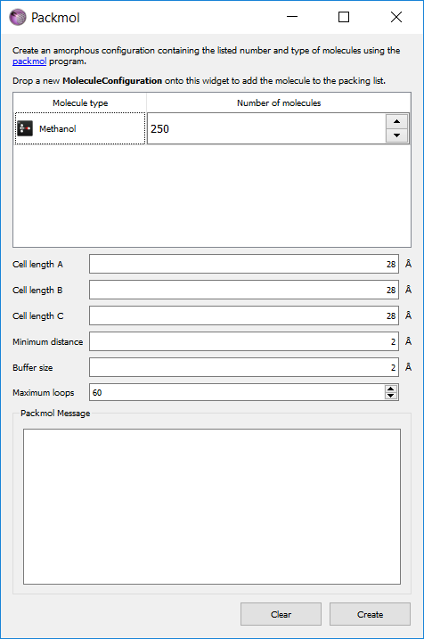
Mouse over the atoms in the new structure to check that the tags reflect the type of each atom.
Adding the forcefield to the calculation
One you are happy with the atom tag assignment, send the bulk methanol structure
to the Scripter  using the Send To icon
  .
.
In the Scripter first add in a ForceFieldCalculator block. In this block the forcefield needs to be defined. To do this a new forcefield definition needs to be added to the script. Open the ForceFieldCalculator and select New. This opens up the Potential Editor dialogue to enter in new forcefield terms.
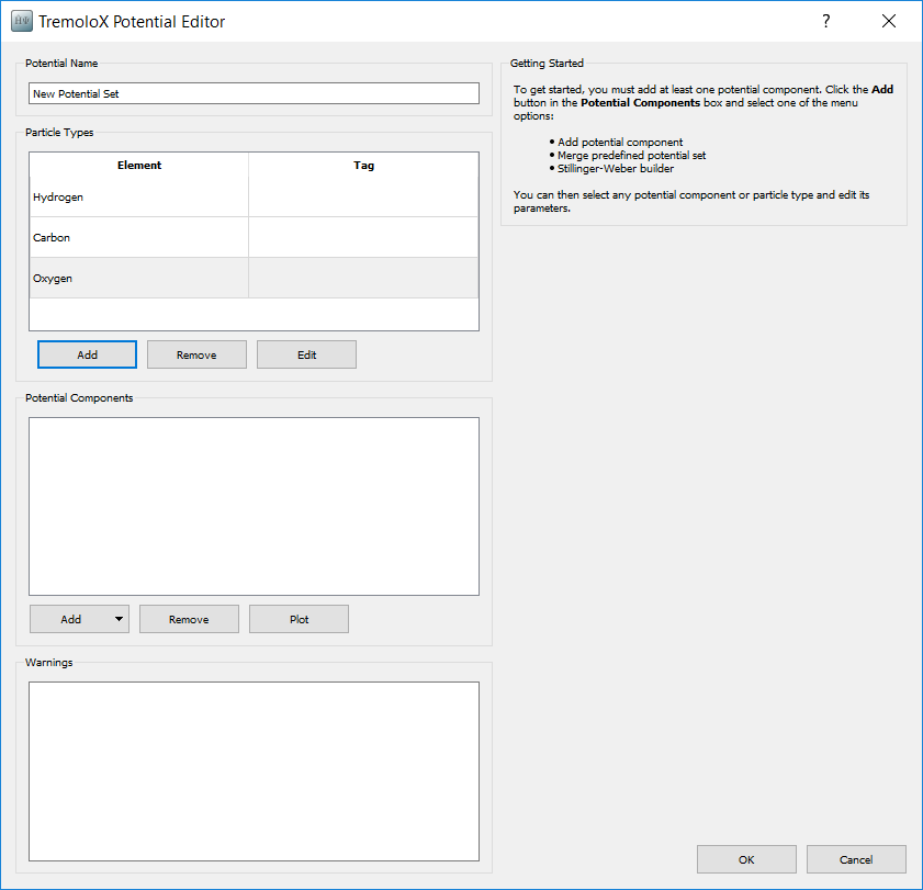
Give the new potential the name Methanol OPLS-AA. When opening the
Potential Editor particle types are added for each atom. These need to be
deleted and replaced with particle types for the 4 atom tags. Select each element
and press Remove. Then press Add to add each atom term.
Atom Tags
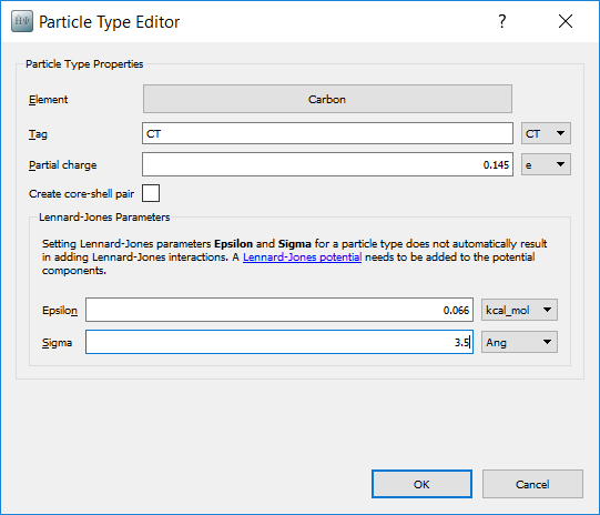
Pressing Add opens the Particle Type Editor. In this the type and basic information about the non-bonding parameters for the type are added.
The OPLS-AA forcefield used the expression for the non-bonding energy \(E_{nb}\):
The terms \(\epsilon_{ij}\) and \(\sigma_{ij}\) are calculed from the Lorentz-Berthelot combination rules:
The nonbonding parameters for the 4 atom types in methanol are:
Type |
\(\epsilon_{i}\) / kcal mol-1 |
\(\sigma_{i}\) / Å |
\(q_{i}\) / e |
|---|---|---|---|
CT |
0.066 |
3.50 |
0.145 |
OH |
0.170 |
3.12 |
-0.683 |
HC |
0.030 |
2.50 |
0.04 |
HO |
0.000 |
0.00 |
0.418 |
Note
The HO type is not a van der Waals site in the OPLS-AA potential, and so the parameters for this atom are zero. It is however an electrostatic site, and so carries a charge.
Select the element from the pop-up periodic table, and then select the tag from the dropdown list. Add the corresponding nonbonding parameters. As an example, the input for the CT type is shown below.
Bonding Terms
Bond stretching energy \(E_{bond}\) is approximated by a simple harmonic spring equation:
There are three different types of bonds in methanol. The parameters for these bonds are given in the following table:
Type I |
Type J |
\(K_{ij}\) / kcal mol-1 Å-2 |
\(r_0\) / Å |
|---|---|---|---|
CT |
OH |
320.0 |
1.41 |
CT |
HC |
340.0 |
1.09 |
OH |
HO |
553.0 |
0.945 |
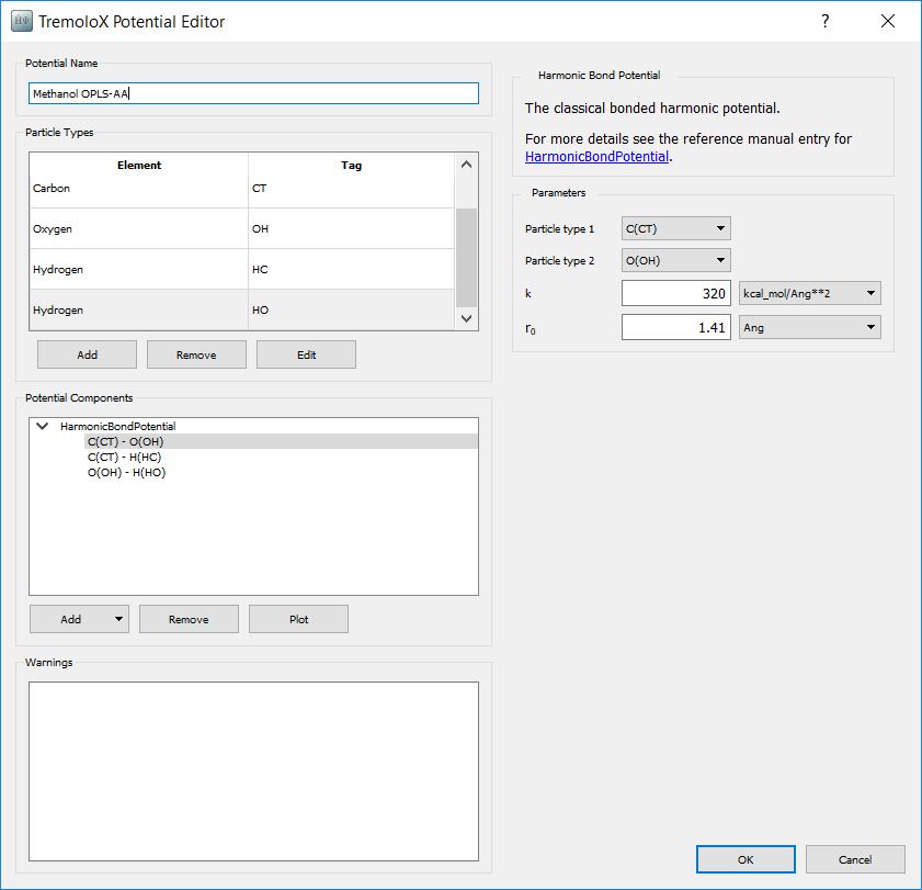
To add the bonding potentials, in the Potential Components box select
. From the list of potential types
select HarmonicBondPotential. Selecting a potential displays the parameters
for it one the right hand side. Add three potentials and enter the parameters
for each bond type. The input for the CT - OH bond type is shown below.
Angle Terms
Angle stretching energy \(E_{angle}\) is approximated by another simple harmonic spring equation:
There are three different types of angles in methanol. The parameters for these angles are given in the following table:
Type I |
Type J |
Type K |
\(K_{ijk}\) / eV rad-2 |
\(\theta_0\) / degree |
|---|---|---|---|---|
CT |
OH |
HO |
2.3861 |
108.5 |
HC |
CT |
OH |
1.5184 |
109.5 |
HC |
CT |
HC |
1.4317 |
107.8 |
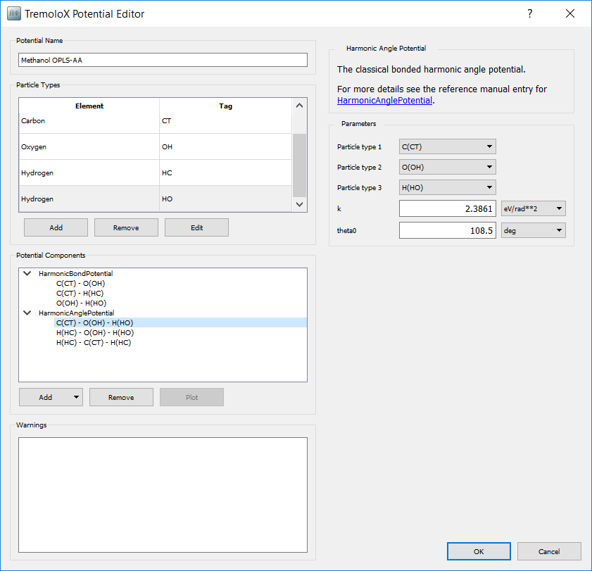
To add the angle potentials, in the Potential Components box select
. From the list of potential types
select HarmonicAnglePotential. Selecting a potential displays the parameters
for it one the right hand side. Add three potentials and enter the parameters
for each bond type. The input for the CT - OH - HO angle type is shown below.
Torsion Terms
In methanol, there is only one bond torsion term. This extends across the type
HC - CT - OH - HO. The bond twisting energy \(E_{torsion}\) in this term
is approximated by a Fourier expansion:
The general torsion term in the OPLS-AA potential is actually a more complicated 3-term Fourier expansion. This potential cannot be added in directly in the interface, but can be easily set up with a small modification to the script. To create a place for the potential, in the Potential Components box select . From the list of potential types select CosineTorsionPotential. We will set the parameters later when editing the final script.
Van der Waals Terms
While parameters have been added for single atom types in the particle type definition, it is also necessary to add terms for pairs of types. As the atom type HO is not a van der Waals site, pair terms involving this atom do not need to be added. The remaining 3 types then gives 6 unique combinations.
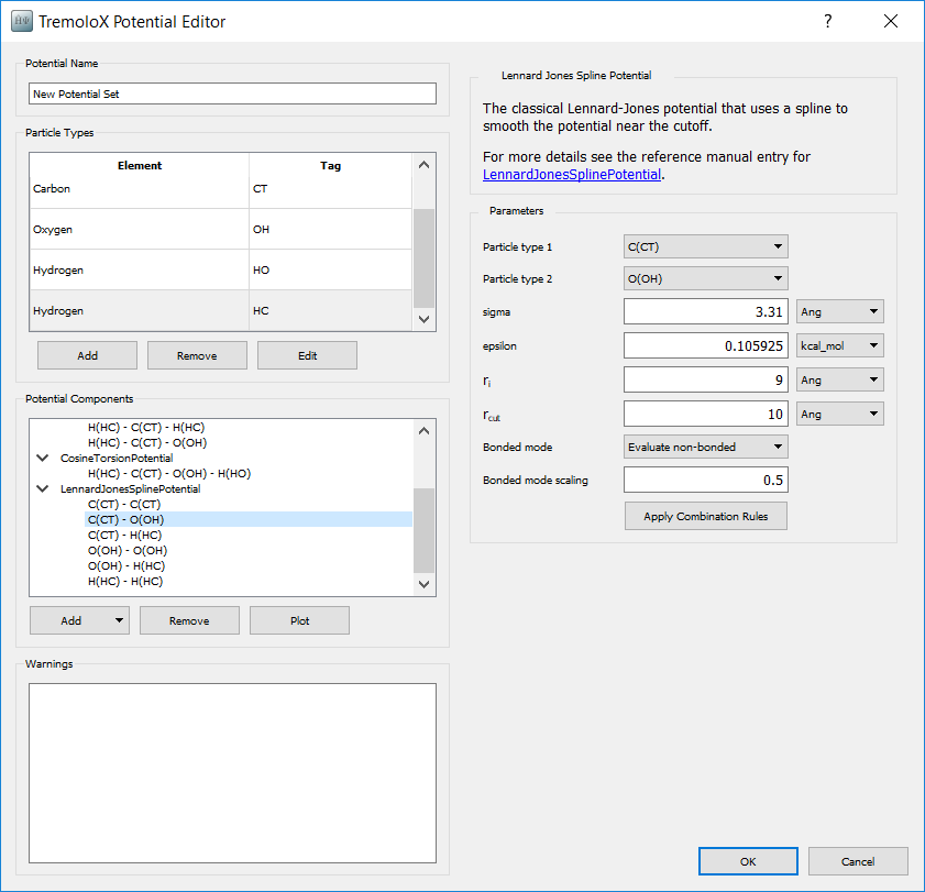
For each combination in the Potential Components box, select . From the list of potential types select LennardJonesSplinePotential. The parameters for each can now be set on the right hand side.
Sigma and epsilon can be filled in from the single atom type parmameters by pushing Apply Combination Rules
Set rcut to
10Å. This sets the distance beyond which potential terms are ignoredSet ri to
9Å. This sets the distance beyond which potential terms are scaled down by a spline function, so that they are zero at the cutoff. This is necessary so that there is not a sudden increase in forces as atoms come within range of each other.Set Bonded mode scaling to
0.5. This scaling is for atoms connected through 3 bonds and is specified by the OPLS-AA potential.
An example for the CT - OH nonbonding potential is shown below.
Electrostatic Terms
Atomic charges were added to the model in the definition of particle types. A summation method for the electrostatic terms still needs to be added.
In the Potential Components box select . From the list of potential types select CoulombSPME. This selects Smooth Particle Mesh Ewald summation of electrostatic terms. This method uses Fourier transforms to correctly estimate the long-range electrostatic interactions.
In the parameters section on the right hand side:
Set rcut to
9Å.Set Accuracy to
0.001.
The other default parameters are suitable for the calculation.
Having added all of these potentials terms, click OK on the Potential Editor and on the ForceFieldCalculator
Relaxing the starting structure
Optimizing the structure
Now that the forcefield has been defined, calculations can be added to the script.
Note
This tutorial follows the general methodology for running molecular dynamics simulations. For more information on specifics of the method and settings see the tutorials:
The first step is to optimise the geometry to remove any large forces from the starting configuration. Large initial forces can cause integration problems in the following molecular dynamics calculations. It is not important that the structure is completely optimised, only that any atom-atom overlaps are removed, which usually happens in the first few steps of a geometry optimisation.
In the Scripter add a block. The default parameters for this block are sufficient.
Obtaining the right density
When the structure was built, the density was too low to make it easier to add methanol molecules into the bulk structure. Now the cell needs to be contracted to approximately the right density. This can be done with a simple molecular dynamics calculation.
Add a molecular dynamics block using the NPT Berendsen barostat. This barostat is more stable but also less accurate than the MTK barostat, making it useful for creating relaxed structures from inital guesses. A run of 100ps is typically sufficient for the system to condense to the liquid density.
Equilibrating the structure
Add a molecular dynamics block using the NPT Martyna Tobias Klein barostat.
In this calculation 100ps is an adequate time for the simulation to equilibrate.
Equilibration time can vary greatly however depending on the system being investigated.
The simulation should also be started using the velocities from the previous calculation,
which can be done by setting the Initial Velocity type to Configuration Velocities.
Setting the production calculation
Add a molecular dynamics block using the NPT Martyna Tobias Klein barostat. Set the dynamics to run for 500ps. The appropriate length of the production simulation depends largely on the system being studied and also the desired accuracy of the final result. Two specific things to that should be set in this part are:
Set the Save Trajectory box to
Production_Trajectory.hdf5Set the Log interval box to 1000
Both of these details will be used in the analysis part of the tutorial.
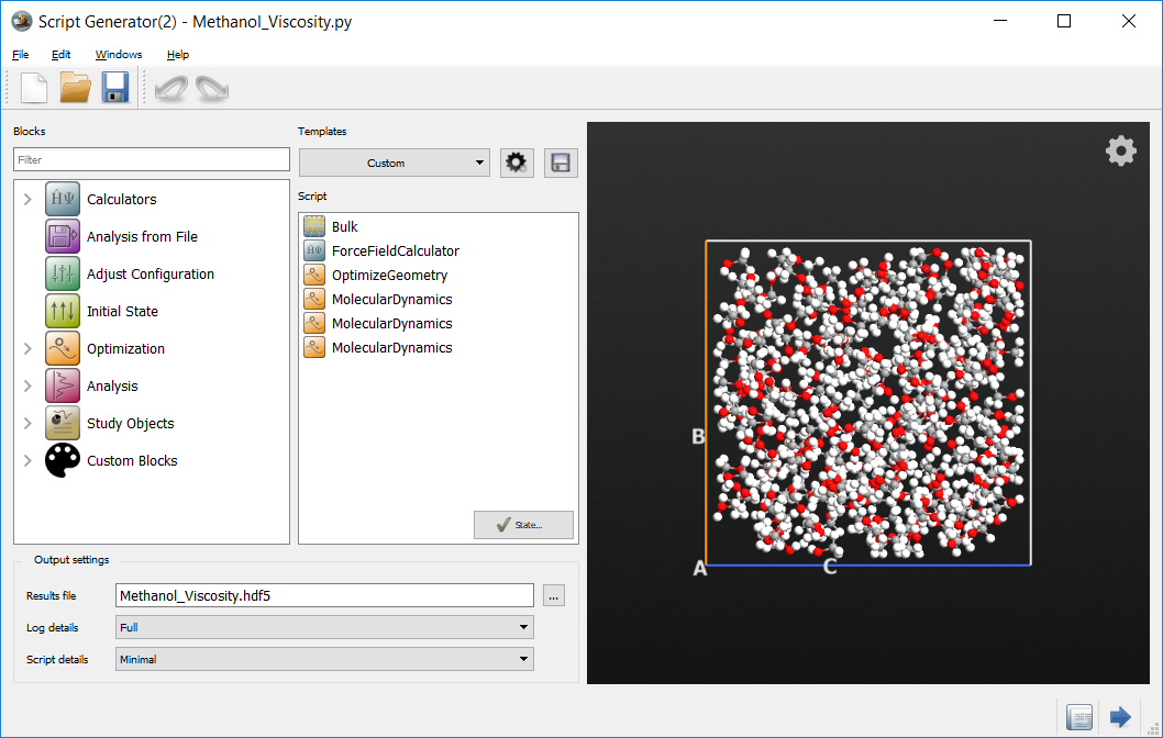
Modifying the script
Adding the torsion terms
Now that the basic calculation is created, Scripter set the output file to
Methanol_Viscosity.hdf5. The script generator should look like:
The script can now be sent to the Editor  using the Send To
icon .
The torsion parameters can now be set. The torsion potential is defined in the
section:
using the Send To
icon .
The torsion parameters can now be set. The torsion potential is defined in the
section:
_potential = CosineTorsionPotential(
   particleType1 = ParticleIdentifier('H', ['HC']),
   particleType2 = ParticleIdentifier('C', ['CT']),
   particleType3 = ParticleIdentifier('O', ['OH']),
   particleType4 = ParticleIdentifier('H', ['HO']),
   k = [0.0*eV, ],
   n = [0, ],
   delta = [0.0*Radians, ],
)
potentialSet.addPotential(_potential)
Replace this block with the block
_potential = CosineTorsionPotential(
   particleType1 = ParticleIdentifier('H', ['HC']),
   particleType2 = ParticleIdentifier('C', ['CT']),
   particleType3 = ParticleIdentifier('O', ['OH']),
   particleType4 = ParticleIdentifier('H', ['HO']),
   k = [0.176*kiloCaloriePerMol, ],
   n = [3, ],
   delta = [0.0*Radians, ],
)
potentialSet.addPotential(_potential)
Save the edited script.
Defining the hook function
To calculate the viscosity the values of the pressure tensor during the simulation are required. As the pressure changes rapidly during the simulation, a high resolution of data is necessary. While saving structures into the trajectory also saves the pressure tensor, saving trajectory files with short timesteps quickly results in unreasonably large files. What is required is a method to save just the pressure information at each step.
In QuantumATK this can be easily achieved with hook functions. These are functions that are run before or after each molecular dynamics integration. Hook functions are designed for either controlling the simulation, or as in this case, recording and analysing various quantities during the simulation.
Note
For an example on how to use hook functions to modify the simulation, see the tutorial: Young’s modulus of a CNT with a defect
To use a hook function a Python object that implements the ‘__call__’ function must first be added. The arguments passed to this function are:
step: The step number that the simulation is up to when the function is called
time: The amount of time that has elapsed in the simulation so far
configuration: A BulkConfiguration object containing the current structure
forces: An array of the forces on each atom
stress: The stress tensor for the current structure
Using these values it is possible to create many custom analysis and data recording methods. In the present case the pressure tensor needs to be recorded. This can be done by the PressureRecordingUtility class defined in the script below.
# Define the class that does the analysis for the MD simulation
class PressureRecordingUtility:
    ''' Calculate and record the volume and pressure tensor at each step '''

    def __init__(self):
        ''' Initialse the arrays used to store the data '''
        self._time_list = []
        self._volume_list = []
        self._pressure_list = []

    def __call__(self, step, time, configuration, forces, stress):
        ''' Function called at each step that calculates and records the pressure tensor '''

        # Add the current time onto the list
        self._time_list.append(time)

        # Get the cell volume and add that to the list too
        volume = configuration.bravaisLattice().unitCellVolume()
        self._volume_list.append(volume)

        # Get the velocity component of the pressure tensor
        velocity = configuration.velocities()
        masses = configuration.atomicMasses()
        velocity_tensor = ((velocity.reshape(-1,3,1) * velocity.reshape(-1,1,3)) * masses.reshape(-1,1,1)).sum(axis=0)

        # Construct the pressure tensor
        pressure_tensor = (velocity_tensor/volume) - stress

        # Add the pressure tensor to the list
        self._pressure_list.append(pressure_tensor)

    def times(self):
        ''' Function that returns the list of times saved during the simulation '''
        return Units.PhysicalQuantity(self._time_list)

    def volumes(self):
        ''' Function that returns the list of volumes saved during the simulation '''
        return Units.PhysicalQuantity(self._volume_list)

    def pressure_tensors(self):
        ''' Function that returns the list of pressure tensors saved during the simulation '''
        return Units.PhysicalQuantity(self._pressure_list)
Paste this code at the top of the simulation script and then save the edited script.
Using the hook function in the molecular dynamics simulation
Now that an appropriate hook function is defined, QuantumATK needs to be told how to use this function during the simulation.
Find the section of the script where the final production phase of the molecular dynamics calculation is carried out. At the top of this section add the following line:
pressureRecorder = PressureRecordingUtility()
This line declares an instance of the class used to record the pressure data, allocating a memory space in which to store it.
Now the MolecularDynamics call needs to be changed to add the hook function. Edit this function call to include the argument:
post_step_hook=pressureRecorder
This tells QuantumATK to use the pressureRecorder instance of the PressureRecordingUtility to run and store the data at each step.
Note
The MolecularDynamics function supports arguments pre_step_hook and post_step_hook for running the hook function before or after the molecular dynamics integration step respectively.
Finally the data collected by the pressureRecorder object needs to be written out to a file for later processing. This can be done by writing the data to a hdf5 file. To do this add the following code to the end of the script.
data_file = 'md_methanol_data.hdf5'
temperature = 300 * Kelvin

nlsave(data_file, pressureRecorder.times(), "Time")
nlsave(data_file, pressureRecorder.pressure_tensors(), "Pressure")
nlsave(data_file, pressureRecorder.volumes(), "Volume")
nlsave(data_file, pressureRecorder.volumes().mean(), "Volume_Average")
nlsave(data_file, temperature, "Temperature")
nlsave(data_file, md_trajectory.timeStep(), "Time_Step")
Save the edited script.
Running the calculation
All of the necessary parts of the script are now in place. The script can be sent
to the Job Manager and run by using the icon.
Analyzing the results
Viewing the change in pressure
When using the NPT ensemble, it is important to check how the pressure was controlled during the simulation. Ideally the pressure should average out to the target value over the course of the simulation. If this does not happen a longer equilibration or simulation time may be needed.
When the NPT ensemble is used the pressure is written to the HDF5 file by default.
To visualise this pressure a script can be used to read it from the HDF5 file
and plot it. To do this open the Editor using the and paste
in the following script.
import pylab

# Read in the existing trajectory to ge the data
trajectory_file = "Production_Trajectory.hdf5"
trajectory = nlread(trajectory_file, MDTrajectory)[-1]
time = trajectory.times()
pressure = trajectory.pressures()

# Set the average and target pressures
p_tot_avg = numpy.cumsum(pressure.inUnitsOf(GPa)) * GPa / (numpy.arange(pressure.shape[0])+1)
p_target = numpy.ones(pressure.shape[0]) * Pa

# Plot the resulting pressure and average pressure
pylab.figure()
pylab.plot(time.inUnitsOf(picosecond), pressure.inUnitsOf(GPa), label='Pressure (GPa)', linewidth=0.5)
pylab.plot(time.inUnitsOf(picosecond), p_tot_avg.inUnitsOf(GPa), label='P Average', linewidth=2.0)
pylab.plot(time.inUnitsOf(picosecond), p_target.inUnitsOf(GPa), label='P Target', linewidth=2.0)
pylab.xlabel('Time (ps)')
pylab.ylabel('Pressure (GPa)')
pylab.legend()
pylab.show()
The script can also be directly downloaded here. pressure_analysis.py
Run this script by sending it to the Job Manager. The script should display a graph similar to the one below.
Tip
Analysis scripts like this can also be run from the command line using the atkpython command
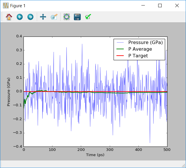
Note that during the dynamics simulation the pressures swing by approximately 0.2GPa. These large pressure changes are typical for molecular dynamics simulations. What is important is that as the simultion runs the average pressure converges to the target pressure of 0.1MPa.
Calculating the viscosity from the Einstein relationship
Using the data collected by the hook function during the molecular dynamics simulation, it is possible to calculate and visualise an estimate of the viscosity.
This can be done by using an ATKPython script. Open a new script in the Editor and paste in the following script.
import pylab
import scipy

# Read the data that is stored in the HDF5 file from the simulation
data_file = 'md_methanol_data.hdf5'
time = nlread(data_file, object_id="Time_8")[-1]
pressure_tensor = nlread(data_file, object_id="Pressure_8")[-1]
volume_avg = nlread(data_file, object_id="Volume_Average_8")[-1]
temperature = nlread(data_file, object_id="Temperature_8")[-1]
time_step = nlread(data_file, object_id="Time_Step_8")[-1]

# Set up the calculation to create 100 time based estimates of the viscosity
N = pressure_tensor.shape[0]
N_steps = 101
skip = int(N/100)
time_skip = time[::skip]

# Calculate the off-diagonal elements of the pressure tensor
P_shear = numpy.zeros((5,N), dtype=float) * Joule / Meter**3
P_shear[0] = pressure_tensor[:,0,1]
P_shear[1] = pressure_tensor[:,0,2]
P_shear[2] = pressure_tensor[:,1,2]
P_shear[3] = (pressure_tensor[:,0,0] - pressure_tensor[:,1,1]) / 2
P_shear[4] = (pressure_tensor[:,1,1] - pressure_tensor[:,2,2]) / 2

# At increasing time lengths, calculate the viscosity based on that part of the simulatino
pressure_integral = numpy.zeros(N_steps, dtype=numpy.float) * (Second * Joule / Meter**3)**2
for t in range(1,N_steps):
    total_step = t*skip

    for i in range(5):
        integral = scipy.integrate.trapz(
            y = P_shear[i][:total_step].inUnitsOf(Joule/Meter**3),
            dx=time_step.inUnitsOf(Second)
        )
        integral *= Second * Joule / Meter**3
        pressure_integral[t] += integral**2 / 5

# Finally calculate the overall viscosity
# Note that here the first step is skipped to avoid divide by zero issues
kbT = boltzmann_constant * temperature
viscosity = pressure_integral[1:] * volume_avg / (2*kbT*time_skip[1:])

# Print the final viscosity
print("Viscosity is {} cP".format(viscosity[-1].inUnitsOf(millisecond*Pa)))

# Display the evolution of the viscosity in time
pylab.figure()
pylab.plot(time_skip[1:].inUnitsOf(ps), viscosity.inUnitsOf(millisecond*Pa), label='Viscosity')
pylab.xlabel('Time (ps)')
pylab.ylabel('Viscosity (cP)')
pylab.legend()
pylab.show()
The script can also be directly downloaded here. viscosity_analysis.py
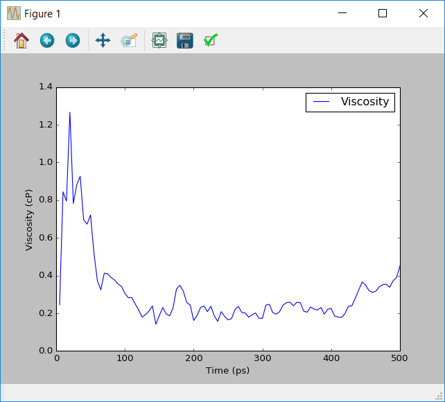
This script reads in the saved data from the HDF5 file saved from the hook function. It then calculates the viscosity using the Einstein relationship given in the theory section. Note that the integral is averaged over the 5 unique off-diagonal components of the pressure tensor, \(P_{xy}\), \(P_{yz}\), \(P_{xz}\), \(\frac{P_{xx}-P_{yy}}{2}\) and \(\frac{P_{yy}-P_{zz}}{2}\). The script then prints the final viscosity at the simulation time limit, as well as showing how the estimate of the viscosity changed over the course of the simulation.
Below is a typical example of the viscosity calculated by the simulation. For comparison the experimental value of the density of methanol at 298K is 0.54cP. A rigid OPLS-AA model which only includes non-bonding interaction and keeps the configuration of each molecule fixed gives a viscosity of 0.43cP[3]. Although the example gives similar results, there is still a reasonable amount of noise in the calcuated viscosity. Ideally this viscosity should converge to a distinct value. This indicates that more sampling of the pressure is required to improve the accuracy of the simulation.
Calculating the viscosity from the Green-Kubo relationship
Similar results for the viscosity can be obtained using the Green-Kubo relationship.
A script outlining how this is achieved can be downloaded here. green_kubo_analysis.py
Advanced users of Python are encouraged to view and run the script to understand how it works. This script also demonstrates some of the power and flexibility of the ATKPython platform for not only running, but also analyzing simulations.
Extending the results
Running more independent trajectories
In the previous section it was seen that more simulations need to be done in order improve the accuracy of the estimated viscosity.
In QuantumATK simulations can be easily repeated by placing them within Python loops. In the case of methanol one strategy is to loop over both the equilibration and production phases of the simulation. As the velocities are re-randomised at the start of the equilibration phase this generates a series of independant trajectories. From these not only the average viscosity but also the error in the average viscosity can be easily estimated using standard statistical methods.
To loop over calculations in Python the code to be repeated can be placed in a for loop. To loop the viscosity calculation 30 times to produce different trajectories the simulation code needs to be placed in a for loop such as:
for loop in range(30):
    # Molecular dynamics simulation commands

# Futher commands outside the loop
Note
One of the important features of Python is that it uses indentation to determine the extent of code blocks. This determines which lines are inside or outside loops and logical statements. The indentation in the above example is how you distinguish code from inside or outside a Python loop.
The only other necessary change in the script to create several trajectories is to modify how the output is done. In HDF5, files writing data with the same text descriptor overwrites the previous data. Unique descriptors are therefore needed. This is simply done by including the looping variable (in the above case the variable loop) into the name. This is done by changing the file-writing code to
data_file = 'md_methanol_data.hdf5'
temperature = 300

nlsave(data_file, pressureRecorder.times(), "Time_"+str(loop))
nlsave(data_file, pressureRecorder.pressure_tensors(), "Pressure_"+str(loop))
nlsave(data_file, pressureRecorder.volumes(), "Volume_"+str(loop))
nlsave(data_file, pressureRecorder.volumes().mean(), "Volume_Average_"+str(loop))
nlsave(data_file, temperature, "Temperature_"+str(loop))
nlsave(data_file, md_trajectory.timeStep(), "Time_Step_"+str(loop))
To read in the data from each trajectory for analysis the names need to be changed
in the nlread commands in the same way.
Improving the accuracy
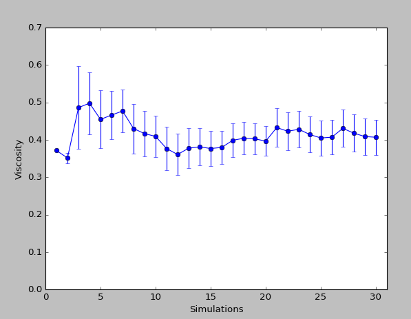
To demonstrate how the accuracy of the simulation can be improved using multiple runs, the simulation was repeated 30 times. The average obtained from these simulations was 0.41cP, with a standard error of 0.05cP. The graph below shows the change in the average viscosity and the standard error with the number of simulations.
References