Noncollinear calculations for metallic nanowires
Version: 2016.3
In the tutorial Introduction to noncollinear spin you learned how to perform a simple noncollinear calculation. In this tutorial you will apply the same procedure to more advanced systems. In a first example, you will consider a metal nanowire connecting two electrodes of the same material. In the second example, you will consider an infinite wire and study the effect of spin-orbit coupling and spin-orientation on the electronic structure. The calculations will be very similar to the two works published by Czerner et al.: [1][2].
Building the device
Set up the Ni(111) surface
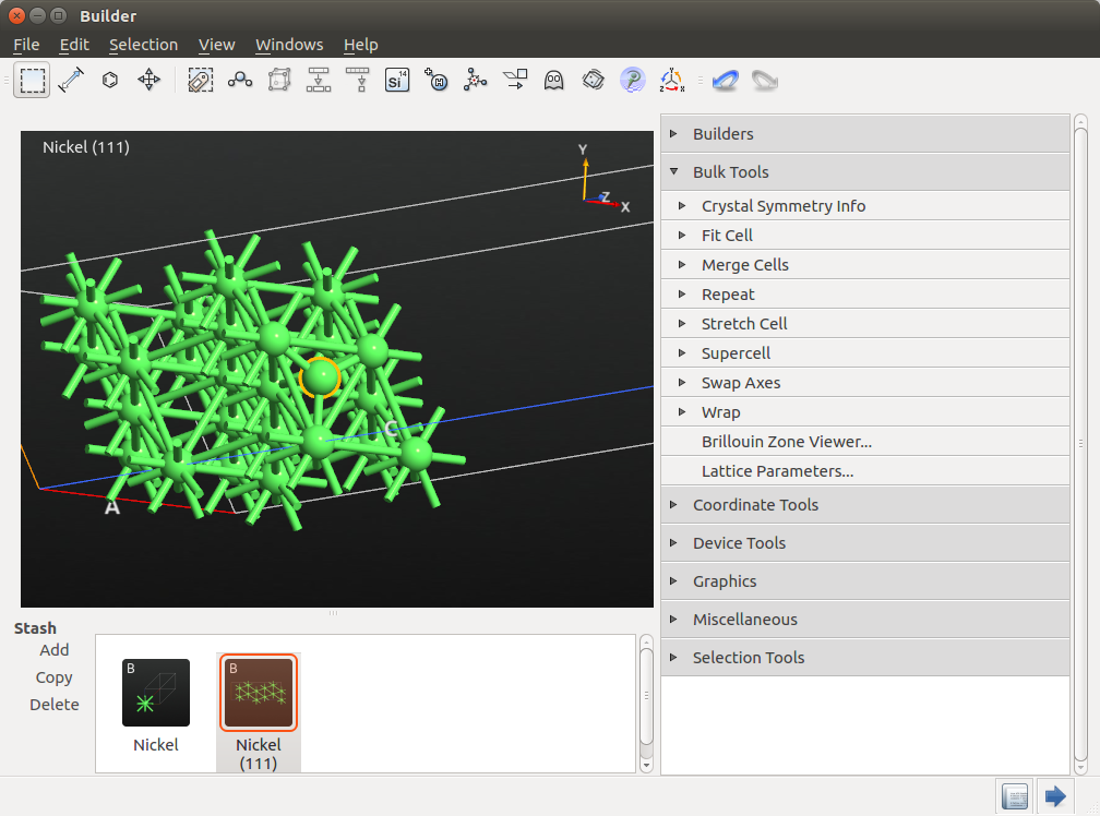
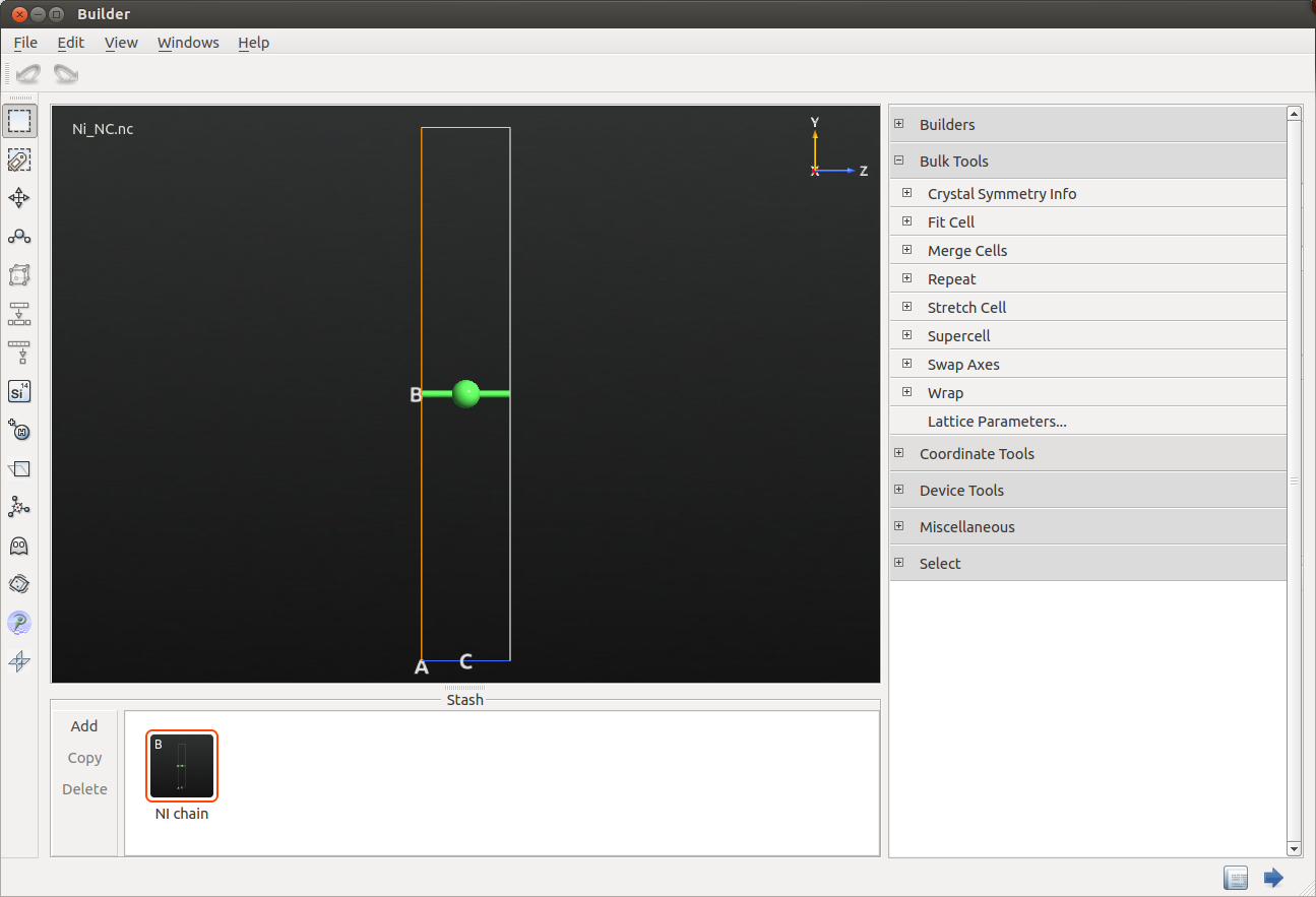
Open the  Builder, click on , search for the Nickel fcc bulk structure and
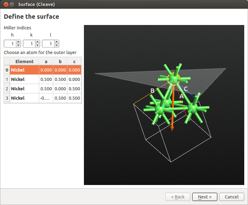
  add it to the Stash. Open , enter Miller indices (111) as shown in the figure below, and click Next.
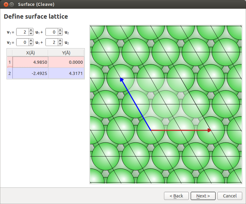
In the next window, define a \(2 \times 2\) surface supercell as shown below, then click Next.
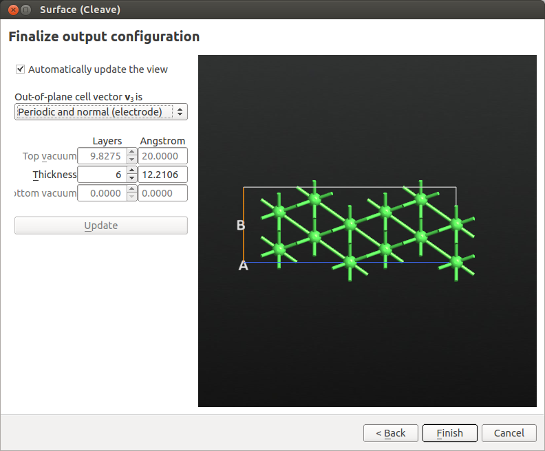
Set the out-of-plane direction to Periodic and normal (electrode), set the thickness to 6 layers (see image below) and click Finish.
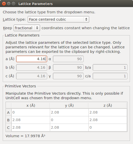
Finally, add some vacuum above the (111) surface. Go to and set the C vector length to 40 Å. Be careful to select to “Keep Cartesian coordinates constant when changing the lattice”.
Note
In principle, you can also create the surface by adding the vacuum in the Surface (Cleave) tool by choosing a slab configuration. The procedure followed here will make the visualization of the next steps easier.
Set up the Ni wire between two Ni(111) surfaces
Select three Ni atoms at the surface and click the centroid plugin on the toolbar at the top of the Builder to add a Ni atom in the geometric center of the selected atoms.
Then, go to to move this atom by 2.035 Å above the surface. This distance corresponds approximately to the Ni(111) interlayer distance.

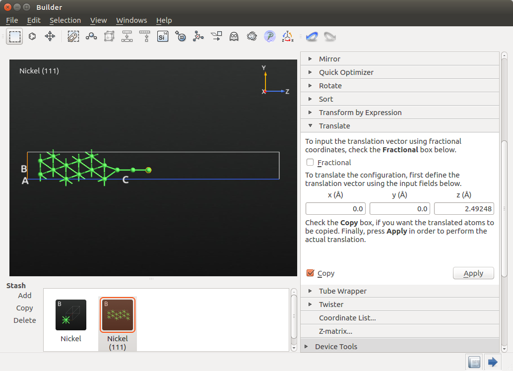
To create the wire, use again but this time select the Copy option and translate by 2.49248 Å, which corresponds to the Ni-Ni distance. Do it twice and you are halfway to creating a 5-atom wire embedded between two Ni electrodes.
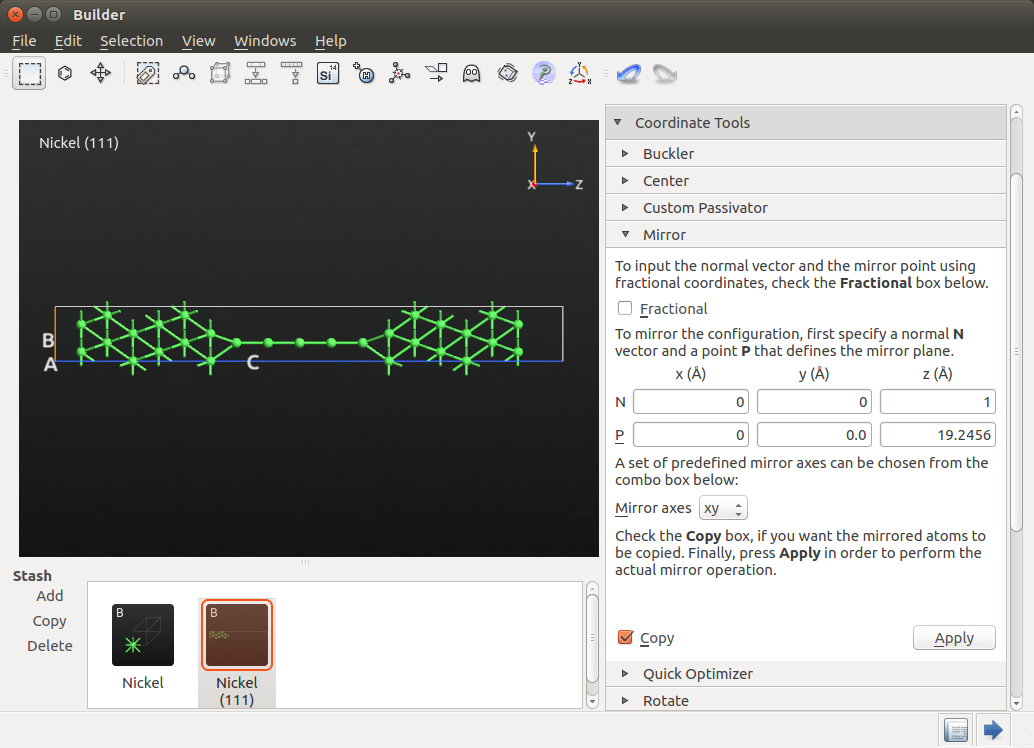
Take note of the Z coordinate of the last Ni atom added to the chain (19.2306 Å) and select all the Ni atoms in your system except this last Ni atom. Then, go to , select the predefined xy mirror axes and enter 19.2306 Å as the Z coordinate of the mirror point P. Remember to check the Copy box to make a copy of the mirrored object, and press Apply and you will obtain the structure shown below.
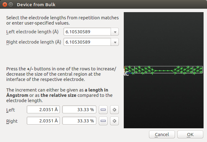
Create the device
Click on and keep the predefined electrode lengths corresponding to three Ni layers.
Setting up the collinear calculation and analyzing the results
In this step you will run a collinear calculation and save the corresponding state in a HDF5 file. In the next step, you will run a noncollinear calculation by using the collinear state as an initial guess. In this way, you will save a lot of computational time, since the convergence of a noncollinear calculation can be hard to achieve otherwise.
Send the device structure you have previously created to the  Script Generator and add the following blocks:
Add a
 New Calculator with the following parameters:
LDA exchange-correlation functional
Spin-polarized calculation
\(4 \times 4 \times 100\) grid for k-points sampling
SingleZetaPolarized basis set
Electron temperature set to 2400 K
Add an
 Initial State with the following options:
Select User spin and check that Spin for Nickel is set to 1.
Add an
 Analysis > MullikenPopulation
Change the output file name to ‘Ni5_collinear.hdf5’.
Note
The high electron temperature considerably improves convergence.
Send the script to the  Job Manager and run the calculation. Once the job is done (in serial it can take up to three hours), the LabFloor will be populated by the
  DeviceConfiguration and
  MullikenPopulation objects.
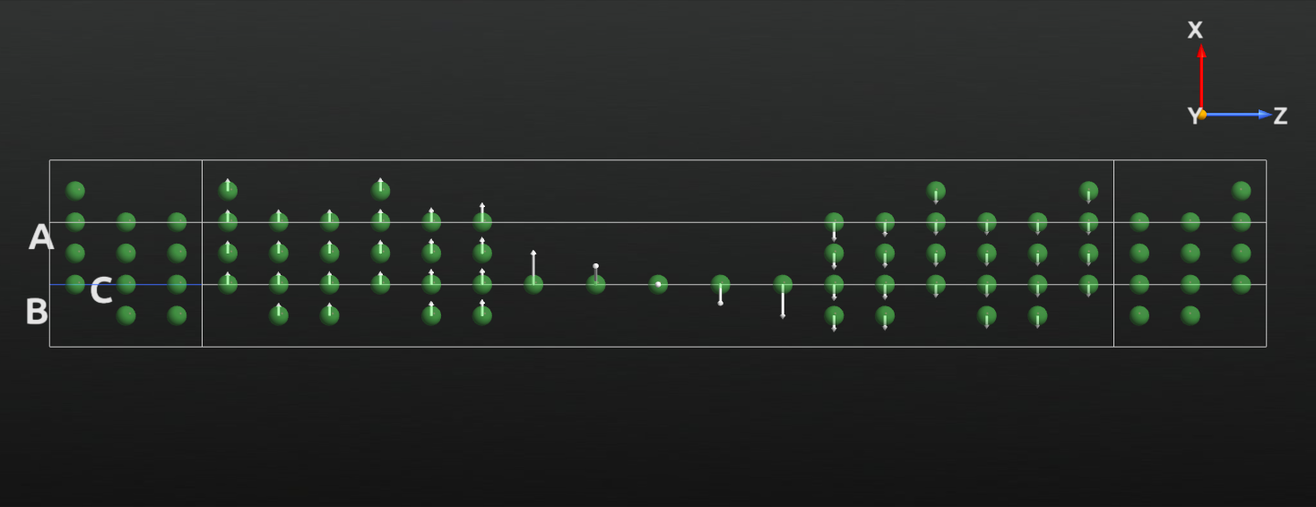
Select the MullikenPopulation and drag and drop it on the  Viewer to visualize the converged collinear spin state.
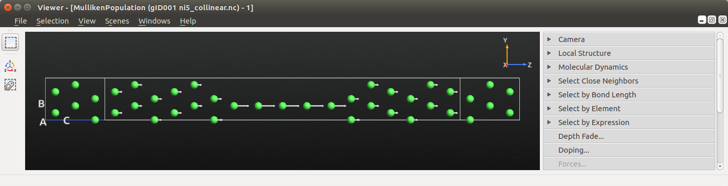
The directions of the arrows is not so interesting or surprising - this is a collinear calculation with the electrodes polarized parallel to each other. We do however see a strong net spin polarization in the atomic wire compared to the surface layers.
Setting up the noncollinear calculation
In the tutorial Introduction to noncollinear spin you have learned how to set up a noncollinear calculation. Here you will learn how to set up the initial spins of a noncollinear calculation based on the collinear converged result.
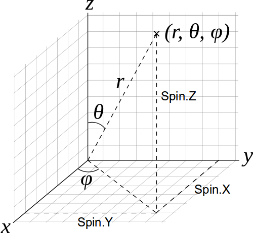
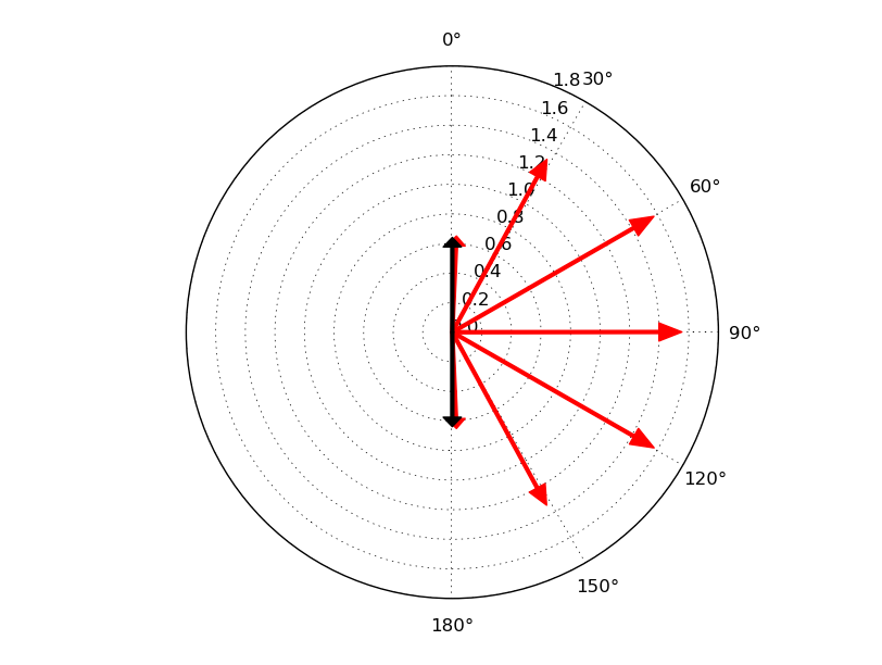
In order to set the initial spin state you need to specify the spin direction in physical spherical coordinates (r, θ, φ), with the following important definitions (see also the figure below):
θ is the angle with the z axis
φ the polar angle in the xy plane relative to the x-axis
Warning
If you start your job by reading a previously converged spin state, as described below in this tutorial, the reference axis (Z in the picture above) for each spin of each atom is the axis of the corresponding converged spin state.
Drag and drop the DeviceConfiguration from the LabFloor to the Script Generator and modify the following parameters:
In the existing
New Calculator, set the spin option to ‘Noncollinear’Add an
Initial State with the following options:Select User spin and check that Spin for Nickel is set to 1
Check the option Use old calculation and use as filename ‘ni5_collinear.hdf5’
Add
Analysis > MullikenPopulation
Send the script to the  Editor and modify the Initial State block as follows:
# -------------------------------------------------------------
# Initial State
# -------------------------------------------------------------

# Define the spin rotation
theta = 180*Degrees
left_spins = [(i, 1, 90*Degrees, 0*Degrees) for i in range(24)]
center_spins = [(i+24, 1, 90*Degrees-theta*(i+1)/6, 0*Degrees) for i in range(5)]
right_spins = [(i+29, 1, 90*Degrees-theta, 0*Degrees) for i in range(24)]
spin_list = left_spins+center_spins+right_spins
initial_spin = InitialSpin(scaled_spins=spin_list)

old_calculation = nlread('ni5_collinear.hdf5', DeviceConfiguration)[0]

device_configuration.setCalculator(
    calculator,
    initial_spin=initial_spin,
    initial_state=old_calculation,
)
device_configuration.update()
nlsave('ni5_noncollinear_out-plane.hdf5', device_configuration)
nlprint(device_configuration)
The setup above corresponds to an out-of-plane spin rotation between two anti-ferromagnetic electrodes, as reported in Refs. [1] and [2] (cf. Figure 1 in Ref. [1]). In a later section you will also consider an in-plane rotation.
Note
The scaled_spin argument follows the format (atom index, initial scaled spin, θ, φ) as documented in the InitialSpin entry in the Reference Manual.
Remember that the spin orientation you enter here is relative to the collinear spin state read before. In this case, the collinear state is ferromagnetic, which corresponds to θ=0 and φ=0.
Save the script in your project directory, check that the ‘ni5_collinear.hdf5’ file is present in the same directory and run the script.
Analyzing the results
Antiparallel configuration, out-of-plane rotation
From the LabFloor drag and drop the MullikenPopulation object contained in ‘Ni5_noncollinear_out-plane.hdf5’ file into the Viewer to visualize the converged noncollinear spin state.
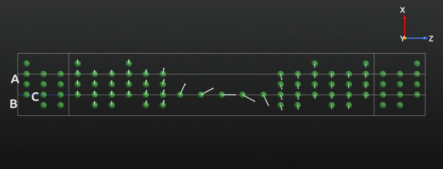
For a more detailed analysis, open the text representation of MullikenPopulation. Here you can read the spin-up, spin-down, θ and φ components for each atom.
The figure below shows the direction and size of the spin state of the atoms in the wire (red arrows) and also of two atoms in the electrode extension regions (black arrows) for comparison. You can compare this plot to the results reported in Refs. [1] and [2].
Antiparallel configuration, in-plane rotation
Another possibility is to rotate the spins in th xy plane by changing the φ angle. To achieve this, modify the script above as indicated below:
# Define the spin rotation
phi = 180*Degrees
left_spins = [(i, 1, 90*Degrees, 0*Degrees) for i in range(24)]
center_spins = [(i+24, 1, 90*Degrees, 0*Degrees+phi*(i+1)/6) for i in range(5)]
right_spins = [(i+29, 1, 90*Degrees, 0*Degrees-phi) for i in range(24)]
spin_list = left_spins+center_spins+right_spins
initial_spin = InitialSpin(scaled_spins=spin_list)
Run the calculation for this initial spin configuration and display the corresponding MullikenPopulation in the Viewer:
Including spin-orbit coupling in noncollinear calculations
ATK also allows you to perform noncollinear calculations including spin-orbit coupling (SOC). In this example, you will investigate the effects of noncollinear spin and spin-orbit coupling to the simple case of an infinite Ni chain [2]. In order to improve the convergence of the calculation, you will first set up a spin polarized calculation and only afterwards perform a noncollinear and finally a calculation with SOC, starting from the previously converged state.
Building the Ni wire
Open the Builder and create a bulk configuration corresponding to an infinite chain of Ni atoms with an interatomic distance of 2.49248 Å (Ni-Ni distance).
Collinear calculation
Send the structure to the Script Generator, and setup the calculation as follows:
Add a
New Calculator with the following parametersPBE exchange-correlation functional
Spin-polarized calculation
\(1 \times 1 \times 13\) k-points sampling
SG15-Medium basis set
- Initial State
Select User spin and check that Spin for Nickel is set to 1.
Change the output file name to ‘ni_collinear.hdf5’.
Note
In order to run a calculation including spin-orbit later on you need fully relativistic pseudopotentials. In this case you will use the SG15 Pseudopotentials and basis sets .
Once you are ready, run the calculation.
Noncollinear calculation with spin-orbit coupling
Drag and drop the DeviceConfiguration contained in the ‘ni_collinear.hdf5’ file from the LabFloor to the Script Generator and modify the following parameters:
In the existing
New Calculator, set the spin option to ‘Noncollinear Spin-Orbit’Add an
Initial StateSelect User spin and check that Spin for Nickel is set to 1.
Check the option Use old calculation and use as filename ‘ni_collinear.hdf5’’
Add
Analysis > BandStructure200 points
G,Z path
Send the script to the Editor and modify the Initial State block as follows:
# -------------------------------------------------------------
# Initial State
# -------------------------------------------------------------

# Define the spin rotation
theta = 0*Degrees
left_spins = [(0, 1, theta, 0*Degrees) ]
initial_spin = InitialSpin(scaled_spins=left_spins)

old_calculation = nlread('Ni_collinear.hdf5', BulkConfiguration)[0]

bulk_configuration.setCalculator(
    calculator,
    initial_spin=initial_spin,
    initial_state=old_calculation,
)
bulk_configuration.update()
nlsave('Ni_noncollinear_phi0.hdf5', bulk_configuration)
nlprint(bulk_configuration)
Then run the calculation. You can notice that in the calculation the direction of the spin is parallel to the C axis (theta=0*Degrees). Once the calculation is done, repeat the calculation by setting the spin direction perpendicular to C (theta=90*Degrees), and compare the two resulting band structures (see figure below).
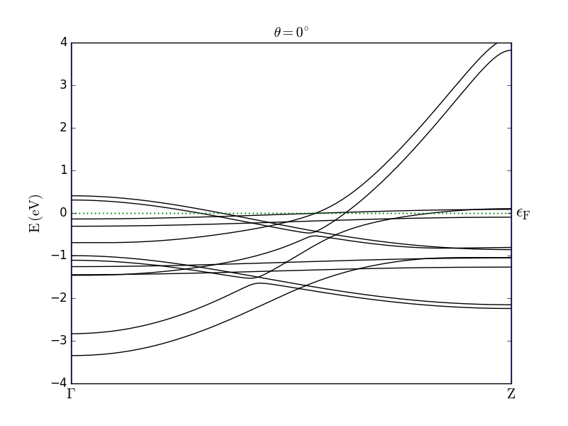
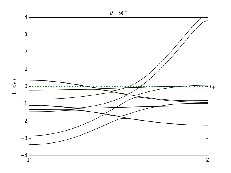
The results are in good agreement with the observations reported in [2]. In particular, the effect of the SOC is clearly visible from the band splitting when the spin is oriented parallel to the wire axis. For both spin orientations you can also observe anticrossing of bands.