\(G_0W_0\) calculator in QuantumATK

In QuantumATK we implemented a \(G_0W_0\) method, which takes initial Kohn-Sham wave functions and energies, and calculates new quasi-particle energies using many-body perturbation theory [1]. In this document, we will try to explain the particular algorithm that is implemented in QuantumATK and how to use it.

Standard GW implementation work purely in imaginary frequency space, and have a scaling with system size of \(O(N^4)\). Recently, an imaginary time to imaginary frequency method has been developed [2], which scales as \(O(N^3)\).

We have combined this approach using an LCAO basis with the PARI approximations as described in [3]. Although it formally scales with system size as \(O(N^3)\), in practice, for small-to-medium sized systems it scales as \(O(N^2)\), since the dominating calculations (polarizability and self-energy) scale as \(O(N^2)\).

Imaginary time and frequency grid

First we need to define the imaginary time and frequency grids \(\{\tau_i, \omega_k\}\). These are optimized to be a non-homogeneous grid to represent MP2 correlation energy as best as possible given an analytic form of the polarizability in imaginary time and frequency:

\[\begin{split}\begin{align*} \eta[\gamma, \omega](x) &= \frac{1}{x} - \frac{1}{\pi}\sum_{k=1}^{N_\omega} \gamma_k \left(\frac{2x}{x^2 + \omega_k^2}\right)^2\\ \eta[\sigma, \tau](x) &= \frac{1}{2x} - \sum_{i=1}^{N_\tau} \sigma_k e^{-2x|\tau_i|} \end{align*}\end{split}\]

The grids are found by minimizing the \(L2\) norm of the cost functions over the range \(x\in[e_{\text{min}},e_{\text{max}}]\) where \(e_{\text{min}}\) is the lowest possible transition and \(e_{\text{max}}\) is the highest.

Optimization is non-linear, and we use a Levenberg-Marquardt algorithm starting from pretabulated initial guesses to find the best possible grid in the interval. This calculation takes up some time, and this is indicated in the log output when running the calculation.

On the GWCalculator, you can use the parameter tau_precision_parameter to influence how many frequency and time points will be used. If the parameter, which is a double, is set to 1.0, the optimization will be done starting from the initial value that contains the most points, which will lead to the most accurate result. If 0.0 is chosen for the parameter, the grid with the least number of points will be chosen. For any value in between an intermediate number of points is selected.

Coulomb integrals and Polarizability using Auxiliary Basis Sets and PARI

The screened (\(W_{\alpha\beta;\gamma\delta}\)) and unscreened (\(V_{\alpha\beta;\gamma\delta}\)) Coulomb integrals, and the polarizability (\(\Pi_{\alpha\beta;\gamma\delta}\)), are 4-index properties. Calculating them directly this way would have unfortunate scaling properties, both for computation time and storage. To avoid this we represent them in auxiliary basis space, in a similar way as in our LCAO-Hybrid code. As auxiliary basis set we use the on-site products of the LCAO basis set, and define the general product of two basis function as:

\[\phi^A_\alpha(\mathbf{r}-\mathbf{R}_A)\phi^B_\alpha(\mathbf{r}-\mathbf{R}_B) = \sum_{M\in[A,B]}\sum_{\mu\in M}C^\mu_{\alpha\beta}P_\mu(\mathbf{r}-\mathbf{R}_M)~,\]

where the auxiliary basis functions, \(P_\mu(\mathbf{r})\) are centered on either of the sites the LCAO basis functions are centered on. This is called the pair-atom resolution of identity (PARI) approximation [4].

If we use this, the Coulomb integral is reduced from a four-index to a two-index quantity:

\[V_{\alpha\beta;\gamma\delta}\approx C^\mu_{\alpha\beta}V_{\mu\nu}C^\nu_{\gamma\delta}\]

Greens functions in imaginary time

Before starting on the actual GW calculation, we do a normal DFT calculation, using any xc-functional. Afterwards, the Greens functions are constructed from the converged Kohn-Sham orbitals, in imaginary time as:

\[G(i\tau)_{\alpha\beta} = \Theta(\tau)~G^+(i\tau)_{\alpha\beta} + \Theta(-\tau)~G^-(i\tau)_{\alpha\beta}~,\]

with

\[\begin{split}\begin{align*} G^+(i\tau)_{\alpha\beta} &= i\sum_{\mathbf{k}n}w_{\mathbf{k}}~f(\epsilon^0_{\mathbf{k}n})\left[\psi_{\mathbf{k}n}^0\right]_\alpha\left[\psi_{\mathbf{k}n}^0\right]_\beta^*e^{-|\epsilon^0_{\mathbf{k}n}-\epsilon^0_F|\tau},\\ G^-(i\tau)_{\alpha\beta} &= i\sum_{\mathbf{k}n}w_{\mathbf{k}}\left[1-f(\epsilon^0_{\mathbf{k}n})\right]\left[\psi_{\mathbf{k}n}^0\right]_\alpha\left[\psi_{\mathbf{k}n}^0(\mathbf{r}')\right]_\beta^*e^{-|\epsilon^0_{\mathbf{k}n}-\epsilon^0_F|\tau}, \end{align*}\end{split}\]

where \(\{\psi^0_{\mathbf{k}n},\epsilon^0_{\mathbf{k}n}\}\) are the solutions to the Kohn-Sham problem. This step scales as \(O(N^3)\) with system size and linearly, \(O(N_k)\), with the number of k-points. Here \(\{\alpha,\beta\}\) are indices for the normal LCAO orbitals.

The number of bands that are included in the Greens function calculation is determined by the input parameter energy_cutoff on the GWCalculator. When the GWCalculator is created it checks the eigenvalues of the DFT calculation in the \(\Gamma\) point, and determines the number of bands that are below the energy_cutoff. These bands are then used in the construction of the Greens functions. This is done because our LCAO basis sets are not made to describe highly excited states, and including all of them might give rise to issues.

Polarizability in imaginary time

The polarizability is defined as a four-index object in function of the Greens function in imaginary time:

\[\Pi_{\alpha\beta;\gamma\delta}(i\tau) = i G^+_{\alpha\gamma}(i\tau) G^-_{\beta\delta}(-i\tau)~.\]

Using the PARI approximation and introducing the auxiliary basis indices as \(\{\mu,\nu\}\) this becomes:

\[\Pi_{\mu\nu}(i\tau) = i \sum_{\alpha\beta}\sum_{\gamma\delta} C^\mu_{\alpha\beta}G^+_{\alpha\gamma}(i\tau) G^-_{\beta\delta}(-i\tau) C^\nu_{\gamma\delta}~.\]

This is a real space object, which for periodic systems has translations that are not included to keep the notation simple. The whole object is Born-von Karman periodic, so that it scales with the k-point sampling chosen by the user. This means that the calculation scales lineary with the number of k-points. If there is no sparsity, the scaling with system size is \(O(N^2)\) because of the PARI approximation, which is much more favorable than the \(O(N^4)\) scaling for this step when calculated directly in frequency space.

Transform from imaginary time to imaginary frequency

We now have the polarizability on an imaginary time grid, but we need it in (imaginary) frequency space to calculate the screened Coulomb potential. Both time and frequency grids are non-homogeneous/non-regular and in order to transform, we need custom transforms.

To get the best possible result we optimize a cosine transform that is optimal to transform the analytic form of the polarizability from time to frequency and back [2], i.e.:

\[\Pi_{\mu\nu}(\omega_k) = \sum_{i=1}^{N_\tau} \gamma_{ki} \cos{\left(\omega_k \tau_i\right)}\Pi_{\mu\nu}(\tau_i)~.\]

with \(\gamma\) chosen to minimize:

\[\eta(x, \gamma) = \frac{2x}{x^2 + \omega_k^2} - \sum_{i=1}^{N_\tau} \gamma_{ki} \cos{\left(\omega_k \tau_i\right)}e^{-x\tau_i}~.\]

Dielectric tensor and screened Coulomb potential

To calculate the dielectric tensor we transform to frequency space and \(\mathbf{k}\) space representation:

\[\epsilon_{\mu\nu}(\mathbf{q},i\omega) = \delta_{\mu\nu} - V^{\frac{1}{2}}_{\mu\kappa}(\mathbf{q})\Pi_{\kappa\lambda}(\mathbf{q}, i\omega)V^{\frac{1}{2}}_{\lambda\nu}(\mathbf{q})\]

The inverse of the dielectric tensor is then used compute the screened coulomb potential:

\[W_{\mu\nu}(\mathbf{q},i\omega) = V^{\frac{1}{2}}_{\mu\kappa}(\mathbf{q})\epsilon^{-1}_{\kappa\lambda}(\mathbf{q},i\omega)V^{\frac{1}{2}}_{\lambda\nu}\]

Once this is calculated for all \(\mathbf{q}\) points we transform back real space and imaginary time:

\[W_{\mu\nu}(\mathbf{q},i\omega)\rightarrow W_{\mu\nu}[\mathbf{T}](i\tau)\]

Exchange and correlation Self-energy calculation

Once we have the screened Coulomb potential, we can use it to calculate the self-energies in imaginary time. But we need to split it up in separate exchange and correlation parts:

\[\Sigma^x_{\alpha\beta} = i \sum_{\gamma\delta}\sum_{\mu\nu}C^\mu_{\alpha\gamma} V_{\mu\nu} C^\nu_{\beta\delta} G^+_{\gamma\delta}(\tau=0)~,\]

and

\[\Sigma^c_{\mu\nu}(\tau) = i \sum_{\gamma\delta}\sum_{\mu\nu}C^\mu_{\alpha\gamma} \tilde{W}_{\mu\nu}(i\tau) C^\nu_{\beta\delta} G_{\gamma\delta}(i\tau)~.\]

where \(\tilde{W} = W - V\). This is done because otherwise \(W(i\omega)\) would not decay in frequency space, and the cosine transform back to \(i\tau\) would be impossible.

This calculation is similar to the one we have in LCAO with Hybrids, the only change is that it needs to be done at all time points. The scaling, for a non-sparse hamiltonian is again \(O(N^2)\) with system size, and since we are using Born-von Karman boundary conditions the scaling with the number of k-points is linear.

This is the point where the heavy calculations end, and if you call update() on the calculator, this is where it stops, and the self-energy will be stored in imaginary time and real space for use in post-processing analysis objects.

Solving the quasi-particle equation to get the band energies

To get the correction to the band energies, we first project the self-energies on the Kohn-Sham bands. For this we Fourier transform the self-energy to the desired k-point and calculate:

\[\Sigma^c_{nn}(\mathbf{k}, i\tau) = \sum_{\alpha\beta}\left[\psi_{\mathbf{k}n}^0\right]_\alpha \Sigma^c_{\alpha\beta}(\mathbf{k},i\tau) \left[\psi^0_{\mathbf{k}n}\right]_\beta~.\]

We can now symmetrize and anti-symmetrize the band self energies and cosine and sine transform them to imaginary frequency space and add them back together:

\[\begin{split}\begin{align*} \Sigma^c_{nn}(\mathbf{k},i\omega) =& \sum_{i=1}^{N_\tau} \gamma_ki \cos{(\omega_k\tau_i)}\left[\Sigma^c_{nn}(\mathbf{k}i\tau) + \Sigma^c_{nn}(\mathbf{k},-i\tau)\right]\\ &+ i\sum_{i=1}\lambda_{ki} \sin{(\omega_k\tau_i)} \left[\Sigma^c_{nn}(\mathbf{k},i\tau) - \Sigma^c_{nn}(\mathbf{k,-i\tau})\right]~. \end{align*}\end{split}\]

To find the correct band-energy for band \(n\) we need to solve the following root-finding problem:

\[\omega = \epsilon^0_n - v^{xc}_n + \Sigma^x_{nn} + \mathrm{Re}\left[\Sigma^c_{nn}(\omega)\right]~,\]

where \(\omega\) is on the real axis now. The \(\omega\) that solves this equation is the \(G_0W_0\) quasi-particle energy. It is important to note that this equation is solved on the real frequency axis. To get the self-energy in real frequency we have to do an analytic continuation, by using the continued fraction representation of the self-energy:

\[\Sigma_{nn}(\omega)\approx \frac{a_1}{1+}\frac{a_2(\omega-\omega_1)}{1+}\ldots\frac{a_{N_\omega}(\omega-\omega_{N\omega-1})}{1+(\omega-\omega_{N_\omega})g_{N_\omega+1}(\omega)}\]

This procedure is in the Analysis objects that are support for GW, which are Bandstructure, DensityOfStates, ProjectedDensityOfStates, FatBandstructure, Eigenvalues and EffectiveMass.

Schematic view of the algorithm

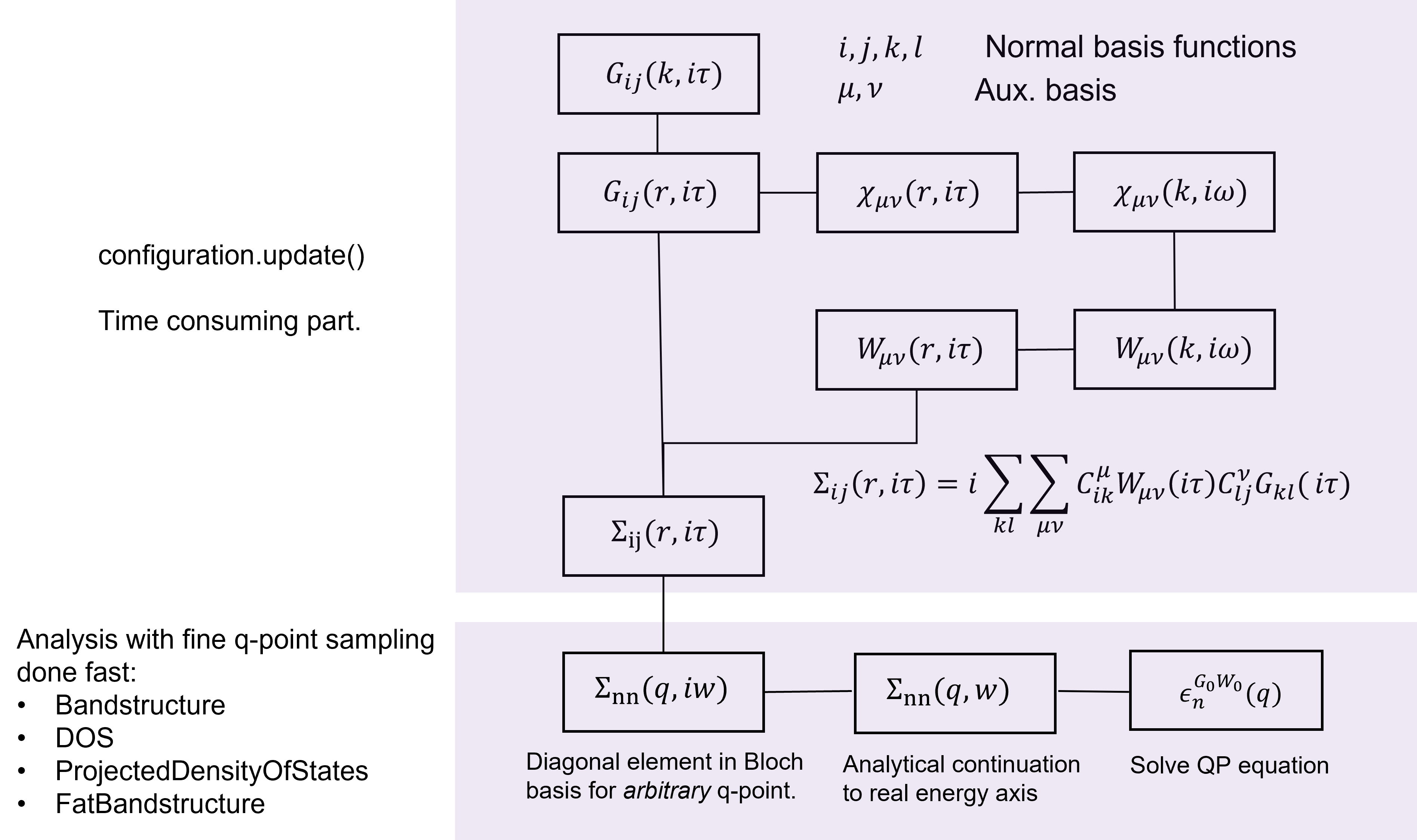
Fig. 215 A flowchart diagram showing how the GW calculations is done, and the quasi-particle energies are calculated.

\(\Gamma\) point correction for k-point convergence

In GW the problem arises that the Coulomb potential needs to be calculated and screened at the \(\Gamma\) point, but this cannot be done since it diverges as \(\frac{1}{q^2}\) for 3D systems and \(\frac{1}{q}\) for 2D systems.

The easiest way to avoid this divergence is just not include the \(\Gamma\) point in the k-point sampling. This can be done by setting include_gamma_point=False on the GWCalculator. The problem is that this will lead to a very slow convergence with k-points for gapped systems, because this assumes that the long range part of the Coulomb potential is perfectly screened by the dielectric tensor, and this will lead to an underestimation of the band gap. To get the correct band gap, one needs to fit a linear curve to the band gap at different k-point sampling, and extrapolate the result to infinite k-point sampling.

We have developed a method to correct for this, both for 3D and 2D systems, so that the contribution at \(\Gamma\) is regularized and the convergence with k-points is much faster, which can be used by setting include_gamma_point=True. This is the default setting in QuantumATK.

In the figures below we show the calculation of the band gap for both 3D Si FCC, and 2D \(\text{MoS}_2\) with and without the \(\Gamma\) point correction, and show that the extrapolated band gap can be approximated well at small k-point sampling using the \(\Gamma\) point correction.

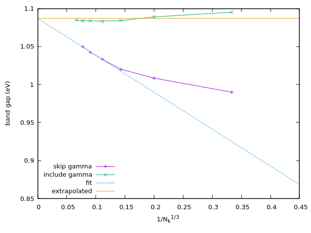
Fig. 216 Si-FCC band gap calculated @PBE with different number of k-points, with and without the \(\Gamma\) point correction.

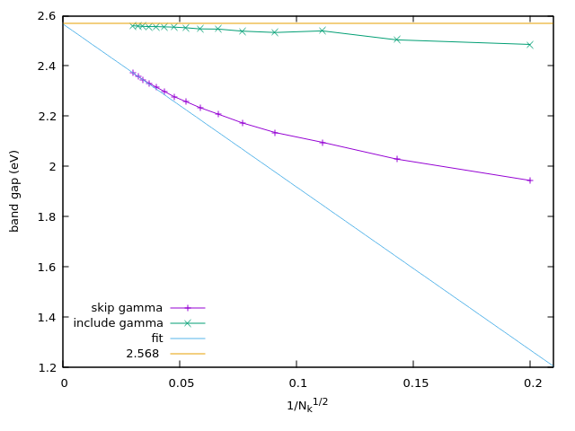
Fig. 217 2D \(\text{MoS}_2\) band gap calculated @PBE with different number of k-points, with and without the \(\Gamma\) point correction.

For metallic systems, the \(\Gamma\) point correction is not important since the long range part of the Coulomb potential is screened by the free electrons. If you are calculating an interface system with both metallic and insulating parts, it is recommended to disable the \(\Gamma\) point correction.

Parallelization of the algorithm

Our implementation of the \(G_0W_0\) method is parallelized using both MPI and openMP. We recommend using openMP threads as much as possible, since it also reduced the memory usage of the calculation. The MPI parallelization of the calculation of the polarizability and self-energy is done over the atoms in the system. It is therefore important to never use more MPI processes than there are atoms in the system you are calculating. Doing so will lead to poor performance.

Usage Examples

To run a GW calculation one first has to construct a regular LCAOCalculator, which is then set on a GWCalculator object:

lcao_calculator = LCAOCalculator(
    basis_set=BasisGGAPseudoDojo.High,
    exchange_correlation=HybridGGA.HSE06)

gw_calculator = GWCalculator(
    lcao_calculator,
    energy_cutoff=50*eV,
    polarizability_compression_parameter=1.0e-07,
    w_compression_parameter=1.0e-05,
    include_gamma_point=True)

bulk_configuration.setCalculator(gw_calculator)
bulk_configuration.update()

Once the update function is called, the self energies are calculated and stored on the GWCalculator object. To get the bandstructure or density of states we just call the standard analysis objects:

bandstructure = Bandstructure(bulk_configuration, bands_above_fermi_level=4)
nlsave("gw_bandstructure.hdf5", bandstructure)

pdos= ProjectedDensityOfStates(
    bulk_configuration,
    MonkhorstPackGrid(21,21,21),
    projections=ProjectOnShellsBySite,
    bands_above_fermi_level=4)
nlsave("gw_pdos.hdf5", pdos)

For GW calculations it is important to have a good basis set. To get a basis set that matches plane-wave accuracy we have developed the BasisSetOptimizer class. For a reference system a plane wave calculation is performed and the LCAO basis set is optimized to match the plane wave calculation. The basis set is then stored in a file:

basis_set_optimizer = BasisSetOptimizer(
    bulk_configuration,
    orbitals_per_shell_map={Silicon: [6,6,5,4]},
    energy_cutoff=10*eV,
    tolerance=1.0e-5)

opt_basis_set = basis_set_optimizer.optimize()
nlsave("opt_basis_set.hdf5", opt_basis_set)

This can be used in the GW calculation by setting it on the LCAOCalculator object:

opt_basis_set = nlread("opt_basis_set.hdf5")[0]
lcao_calculator = LCAOCalculator(
    basis_set=opt_basis_set,
    exchange_correlation=HybridGGA.HSE06)

gw_calculator = GWCalculator(
    lcao_calculator,
    energy_cutoff=50*eV,
    polarizability_compression_parameter=1.0e-07,
    w_compression_parameter=1.0e-05,
    include_gamma_point=True)

bulk_configuration.setCalculator(gw_calculator)
bulk_configuration.update()

References

[1]

Giovanni Onida, Lucia Reining, and Angel Rubio. Electronic excitations: density-functional versus many-body Green’s-function approaches. Rev. Mod. Phys., 74:601–659, Jun 2002. URL: https://link.aps.org/doi/10.1103/RevModPhys.74.601, doi:10.1103/RevModPhys.74.601.

[2] (1,2)

Peitao Liu, Merzuk Kaltak, Jiri Klimes, and Georg Kresse. Cubic scaling GW: Towards fast quasiparticle calculations. Phys. Rev. B, 94:165109, Oct 2016. URL: https://link.aps.org/doi/10.1103/PhysRevB.94.165109, doi:10.1103/PhysRevB.94.165109.

[3]

Xinguo Ren, Florian Merz, Hong Jiang, Yi Yao, Markus Rampp, Hermann Lederer, Volker Blum, and Matthias Scheffler. All-electron periodic G0W0 implementation with numerical atomic orbital basis functions: Algorithm and benchmarks. Phys. Rev. Mater., 5:013807, Jan 2021. URL: https://link.aps.org/doi/10.1103/PhysRevMaterials.5.013807, doi:10.1103/PhysRevMaterials.5.013807.

[4]

Peize Lin, Xinguo Ren, and Lixin He. Efficient Hybrid Density Functional Calculations for Large Periodic Systems Using Numerical Atomic Orbitals. Journal of Chemical Theory and Computation, 17(1):222–239, 2021. PMID: 33307678. URL: https://doi.org/10.1021/acs.jctc.0c00960, arXiv:https://doi.org/10.1021/acs.jctc.0c00960, doi:10.1021/acs.jctc.0c00960.