Introduction to Array Jobs
Often, one wants to run many similar calculations in parallel. Perhaps one wants to scan over a specific set of parameters or calculate specific properties for many different structures.
One way to achieve this is to take advantage of the array jobs feature present in all standard HPC queueing systems such as PBS, LFS or SLURM. Instead of performing all the calculations in one single, huge job an array job allows the queuing system to manage the computation in a much more fine-grained way, where each of the many calculations are only submitted in smaller batches whenever sufficient resources are available. This often leads to much faster computation times, since the job does not have to wait for a single large reservation of computing resources to become available.
While running array jobs comes with a a lot of advantages, they are also much harder to set up and submit compared to regular jobs. Also, once the computation has finished, it is also much harder to gather the data of all the independent calculations.
The QuantumATK Workflow Builder and Jobs tool now takes away all the hassle of setup, submission and data gathering for array jobs. They are now essentially as easy to set up as normal computation jobs.
This small guide shows you how you can leverage the power of array jobs in QuantumATK.
Table of Contents

How to build an array script in the Workflow Builder
We begin by using the Workflow Builder to set up an array script.
As a quick example, let us imagine that we are interested in Silicon and wish to investigate Silicon using a LCAOCalcualtor. An important first step is then to converge the density mesh cut-off for the LCAOCalculator. We can do this by calculating the Total Energy of the Silicon system for different values of the density mesh cut-off, and all these independent calculations can be performed in an array job.
Let us set up the following workflow:
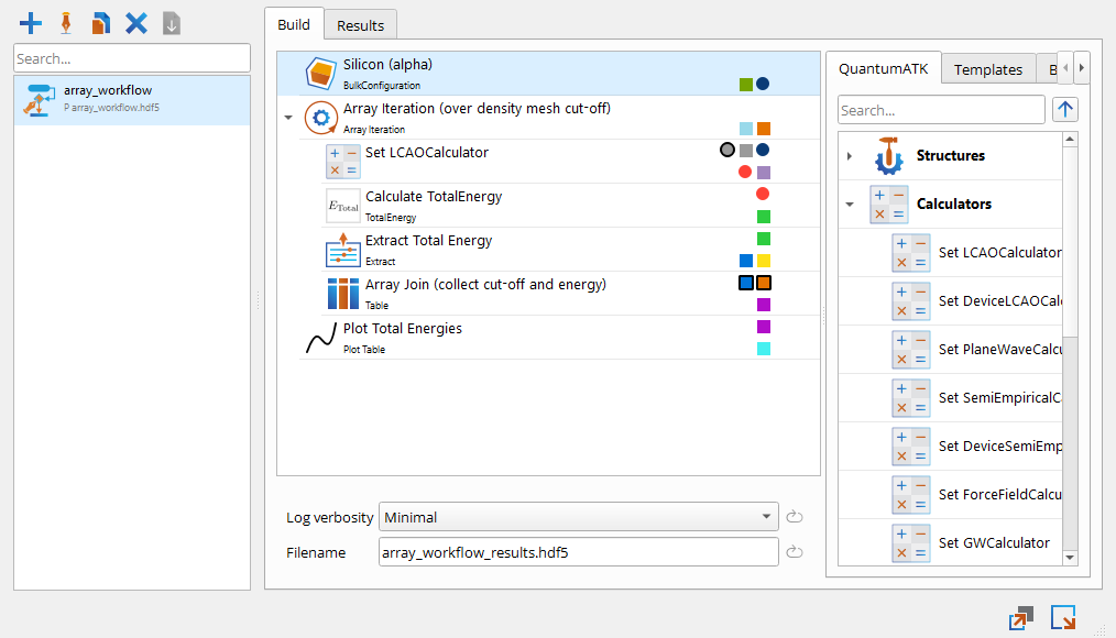
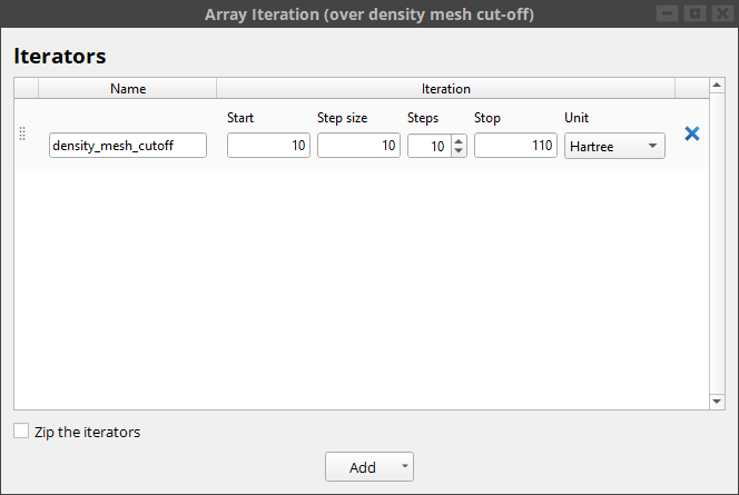
The array iteration block creates a density_mesh_cutoff variable that iterates over energies of 10, 20, …, 110 Hartree.
Tip
Array jobs can be built using either the Array iteration block or the Array table iteration block.
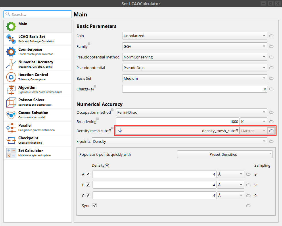
The density_mesh_cutoff variable is then plugged into the LCAOCalculator block.
All array jobs must collect their result in a Table. In this case we save both the input density mesh cut-off and the resulting total energy in the table.
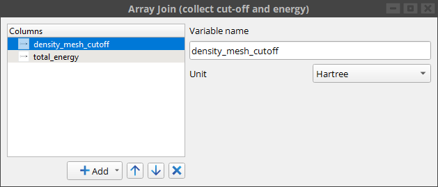
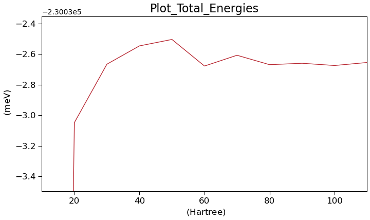
Note that the workflow also contains a plot of the total energy against the density mesh cut-off, so it is straight forward to gauge the convergence.
Next, in the lower right corner of the Workflow Builder we then click the “Arrow” and then select “Editor as Array script”. The resulting script looks like this:
# ARRAY prepare 11 finalize

import itertools

# Set minimal log verbosity
setVerbosity(MinimalLog)

results_filename = 'array_workflow_results.hdf5'

# Extract array part (if present).
part = os.environ.get('PART')
common_folder = os.getcwd()

# Common setup.
if part in ('prepare', None):
    # Set up lattice
    lattice = FaceCenteredCubic(5.4306*Angstrom)

    # Define elements
    elements = [Silicon, Silicon]

    # Define coordinates
    fractional_coordinates = [[ 0.  ,  0.  ,  0.  ],
                              [ 0.25,  0.25,  0.25]]

    # Set up configuration
    silicon_alpha = BulkConfiguration(
        bravais_lattice=lattice,
        elements=elements,
        fractional_coordinates=fractional_coordinates
        )

    silicon_alpha_name = "silicon_alpha"

    nlsave(results_filename, silicon_alpha, object_id='silicon_alpha')

# Parallelize.
if part in ('main', None):
    if part == 'main':
        # Extract array specifics.
        folder = os.environ['ARRAY_FOLDER']
        array_index = int(os.environ['ARRAY_INDEX'])
        array_size = int(os.environ['ARRAY_SIZE'])
    else:
        folder = '.'
        array_index = None
        array_size = None

    # Move to the array folder.
    os.chdir(folder)

    silicon_alpha = nlread(
        os.path.join(common_folder, results_filename), object_id='silicon_alpha'
    )[0]

    # Array Iteration (over density mesh cut-off)(preparation)
    ############################################################
    #          Array Iteration (density_mesh_cutoff)           #
    ############################################################

    # Create iterator.
    def densityMeshCutoffsIterator():
        for i in range(11):
            v = (10.0 + i * 10.0) * Hartree
            yield v

    density_mesh_cutoffs = densityMeshCutoffsIterator()

    def arraySplit(generator, length, array_size, array_index):
        """
        Determine the start and end indices to distribute an generator over
        an array of calculations.

        :param length:          The length of the generator.
        :type  length:          int

        :param array_size:      The array length.
        :type  array_size:      int

        :param array_index:     The array index.
        :type  array_index:     int

        :returns:               An generator over the split indices.
        :rtype:                 iterator
        """
        # Fallback if no array parameters were set.
        if None in (array_size, array_index):
            return generator

        size = length // array_size
        extra = length % array_size

        start = array_index * size + min(array_index, extra)
        stop = (array_index + 1) * size + min(array_index + 1, extra)

        return itertools.islice(generator, start, stop)

    for density_mesh_cutoff in arraySplit(
        density_mesh_cutoffs, 11, array_size, array_index
    ):

        # %% Set LCAOCalculator

        # %% LCAOCalculator

        k_point_sampling = KpointDensity(
            density_a=4.0 * Angstrom, density_b=4.0 * Angstrom, density_c=4.0 * Angstrom
        )

        numerical_accuracy_parameters = NumericalAccuracyParameters(
            density_mesh_cutoff=density_mesh_cutoff, k_point_sampling=k_point_sampling
        )

        calculator = LCAOCalculator(
            numerical_accuracy_parameters=numerical_accuracy_parameters,
            checkpoint_handler=NoCheckpointHandler,
        )

        # %% Set Calculator

        silicon_alpha.setCalculator(calculator)

        silicon_alpha.update()

        # %% Calculate TotalEnergy

        calculate_total_energy = TotalEnergy(configuration=silicon_alpha)

        # %% Extract Total Energy

        def extract_total_energy(total_energy):
            evaluate = total_energy.evaluate()
            return evaluate

        evaluate = extract_total_energy(calculate_total_energy)

        # %% Array Join (collect cut-off and energy)

        if 'array_join_collect_cutoff_and_energy' not in locals():
            array_join_collect_cutoff_and_energy = Table(
                results_filename, object_id='table'
            )
            array_join_collect_cutoff_and_energy.addQuantityColumn(
                key='density_mesh_cutoff', unit=Hartree
            )
            array_join_collect_cutoff_and_energy.addQuantityColumn(
                key='total_energy', unit=eV
            )
            array_join_collect_cutoff_and_energy.setMetatext(
                'Array Join (collect cut-off and energy)'
            )

        array_join_collect_cutoff_and_energy.append(density_mesh_cutoff, evaluate)

# Collect all results into common table.
if part in ('collect', 'finalize'):
    # Extract array specifics.
    array_folder_prefix = os.environ['ARRAY_FOLDER_PREFIX']
    array_size = int(os.environ['ARRAY_SIZE'])

    # Collect all tables into one.
    if part == 'finalize':
        array_join_collect_cutoff_and_energy = Table(results_filename)
    else:
        array_join_collect_cutoff_and_energy = Table('partial_' + results_filename)

    for array_index in range(array_size):
        path = os.path.join(array_folder_prefix + str(array_index), results_filename)

        try:
            # Read the partial table.
            partial_table = nlread(path, object_id='table')[0]

            # Extend main table.
            array_join_collect_cutoff_and_energy.extend(partial_table)
        except Exception:
            print(f'No file found for index {array_index} at {path}.')

# Post-process results.
if part in ('collect', 'finalize', None):

    # Create PlotModel.
    plot_model = Plot.PlotModel(x_unit=Hartree, y_unit=meV)

    plot_model.framing().setTitle('Plot_Total_Energies')

    # Add line
    Total_energy = Plot.Line(
        array_join_collect_cutoff_and_energy[:, 'density_mesh_cutoff'],
        array_join_collect_cutoff_and_energy[:, 'total_energy'],
    )
    Total_energy.setLabel('Total energy')
    Total_energy.setColor('#b82832')
    Total_energy.setLineStyle('-')
    Total_energy.setMarkerStyle('')
    plot_model.addItem(Total_energy)

    # Auto-adjust axis limits.
    plot_model.setLimits()

    # Save plot to file.
    Plot.save(plot_model, results_filename)
This script effectively splits the calculation up into three different parts. First a common “prepare” part that sets up the silicon structure, then an “array” part that calculates the total energy for the different density mesh cut-offs and lastly a “finalize” part, in which the array results are collected and plotted.
This script is specifically adapted to work with the QuantumATK Jobs tool. However, it is also made in such a way that it will still work when submitted as a normal job. Running it like a normal job will of course be a lot less efficient, as it will run entirely in a single process. It is also possible to prepare your own array scripts for submission with the Jobs tool by using e.g. the example script above as a template.
Once the script is created, save it in preparation for submitting it in the Jobs tool.
How to submit an array script
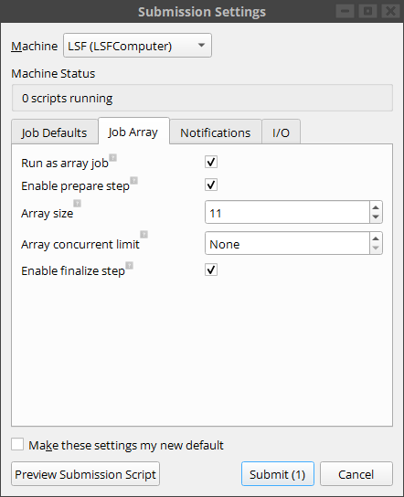
Start by sending the array script to the Jobs tool. In the job creation dialog choose a machine with a queueing system, e.g. LSF, SLURM or PBS.
The submission dialog contains a specific tab for array jobs settings. Note that this tab has already been filled out with the relevant information taken from the first comment line in the array script.
Creating the job and pressing submit, we can follow the progress of the job in log panel. In our case it would look like this:
+------------------------------------------------------------------------------+
| Total Array Jobs                                                             |
+------------------------------------------------------------------------------+
| Total jobs:                 13                                               |
| Queued jobs:                 1                                               |
| Running jobs:                7                                               |
| Completed jobs:              5                                               |
+------------------------------------------------------------------------------+

+------------------------------------------------------------------------------+
| Progress                                                                     |
+------------------------------------------------------------------------------+
| Running      [***************************                       ]            |
| Completed    [*******************                               ]            |
+------------------------------------------------------------------------------+

+------------------------------------------------------------------------------+
| Job status                                                                   |
+------------------------------------------------------------------------------+
| Prepare                     Done                                             |
| Main 0                      Done                                             |
| Main 1                      Done                                             |
| Main 2                   Running                                             |
| Main 3                   Running                                             |
| Main 4                   Running                                             |
| Main 5                   Running                                             |
| Main 6                   Running                                             |
| Main 7                   Running                                             |
| Main 8                   Running                                             |
| Main 9                      Done                                             |
| Main 10                     Done                                             |
| Finalize                  Queued                                             |
+------------------------------------------------------------------------------+
Tip
The array log files are each put in separate folders, and they can be inspected in the special log files tab.
When the calculations have finished all the main results are downloaded. This includes all outputs from the main part of the workflow, i.e. all results form the prepare and finalize parts and the table from the array part. The created plot looks like this, showing a convergence to less then 1 meV at around 30 Hartree.