Spin Transfer Torque
Version: 2016.3
In this tutorial you will learn about the spin transfer torque (STT) and how to calculate the STT in magnetic tunnel junctions.
We will use a simple model of such a tunnel junction; a magnetic carbon-chain device. The QuantumATK package offers a convenient analysis object for calculating STT linear-response coefficients at zero bias, but you will also calculate the STT using finite-bias calculations and compare results to those obtained using linear response.

Introduction
Spin transfer torque occurs in situations where a current of spin-polarized carriers from the left part of a device with a particular polarization (given by the unit vector \(S_1\)) enters the right part of the device with a different magnetization direction (given by the unit vector \(S_2\)). When the electrons incoming from the left side enter the right magnetic part, they will eventually be polarized along \(S_2\), meaning that the right magnetic domain has exerted a torque on the electrons in order to rotate their spin angular momentum. However, due to conservation of angular momentum, the electrons exert an equal but opposite torque on the right magnetic domain – the spin transfer torque. Note that a noncollinear description of electron spin is needed to study this effect!
Application in Random Access Memory (RAM)
The spin transfer torque can be used to modify the orientation of a magnetic layer in a magnetic tunnel junction (MTJ) by passing a spin-polarized current through it, and can therefore be used to flip the active elements in magnetic random-access memory (MRAM).

Theory
There are two principally different ways to calculate STT from atomic-scale models:
The STT can be found from the divergence of the spin current density, \(\nabla \cdot I_s\), which in QuantumATK can be directly calculated using Green’s function methods.
Another way to calculate the STT, here denoted \(\bf{T}\), is from the expression \(\bf{T} = \bf{Tr} ( \delta \rho_\mathrm{neq} \bf{\sigma} \times \bf{B_\mathrm{xc}} )\), where \(\delta \rho_\mathrm{neq}\) is the non-equilibrium contribution to the density matrix, \(\bf{\sigma}\) is a vector of Pauli matrices, and \(\bf{B_\mathrm{xc}}\) is the exchange-correlation magnetic field.
Method 2 will be used in this tutorial. We can either calculate \(\delta \rho_\mathrm{neq}\) from the difference between finite-bias and zero-bias calculations, \(\delta \rho_\mathrm{neq} = \rho_\mathrm{neq} - \rho_\mathrm{eq}\), or we can estimate it using linear response theory, \(\delta \rho_\mathrm{neq} = (G^\mathrm{r} \Gamma_\mathrm{L} G^\mathrm{a})qU\), where \(G^\mathrm{r/a}\) is the retarded/advanced Green’s function, \(\Gamma_\mathrm{L}\) is the left-electrode coupling operator, \(U\) is the bias voltage, and \(q\) is the electron charge. The expression for the STT given in method 2 above is then evaluated in real space.
ATK implements a convenient analysis object for calculating the spin transfer torque using method 2 in the linear-response approximation, where the non-equilibrium density response depends linearly on the bias.
Getting Started
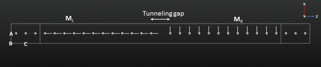
You will here consider a device configuration consisting of a carbon chain with a gap in the middle, which the electrons have to tunnel through. The system is highly artificial, but serves as a simple model of a magnetic tunnelling junction.
Note
There is no need for k-point sampling in the A- and B-directions in this 1D device. However, for commonly studied magnetic tunnelling junctions, like Fe|MgO|Fe, a very fine k-point sampling along A and B is often needed.
Collinear Initial State
The 1D carbon-chain device illustrated above is similar to the one used
in the tutorial Introduction to noncollinear spin, but not identical to it.
Download the device configuration as an QuantumATK Python script: device.py.
As already mentioned, a noncollinear representation of the electron spin is needed
when calculating STT. We will use a collinear, spin-parallel ground state as
initial guess for the noncollinear state.
First step is therefore a collinear calculation for the 1D device.
Send the geometry to the  Script Generator and set up
the ATK-DFT calculation:
Script Generator and set up
the ATK-DFT calculation:
Set the default output file to
para.nc.Add a
 New Calculator block and set the Spin to Polarized.
The exchange-correlation functional will automatically switch to LSDA.
Change the carbon basis set to SingleZetaPolarized in order to speed up
calculations.
New Calculator block and set the Spin to Polarized.
The exchange-correlation functional will automatically switch to LSDA.
Change the carbon basis set to SingleZetaPolarized in order to speed up
calculations.Add an
 Initial State block and select User spin in order
to initialize the calculation with all carbon atoms maximally polarized.
Initial State block and select User spin in order
to initialize the calculation with all carbon atoms maximally polarized.
Save the script as para.py (it should look roughly like this: para.py),
and run the calculation using the  Job Manager.
Noncollinear State: 90° Spin Rotation
Next step is a noncollinear calculation where the spins on the left side of the tunnelling gap point in a different direction than the spins on the right side of the gap. The basic recipe to do this is fairly simple:
The ATK-DFT calculator settings used in the collinear calculation, saved in
para.nc, are loaded from file and slightly adapted for the noncollinear calculation.The spins in the right-hand part of the device are rotated 90° around the polar angle \(\theta\).
The spin-parallel collinear ground state is used as initial state for the noncollinear calculation.
The QuantumATK Python script shown below implements the basic steps given above, but also runs a Mulliken population analysis for visualizing the resulting spin directions throughout the device, and computes the electrostatic difference potential (EDP) and the transmission spectrum.
 1# Read in the collinear calculation
 2device_configuration = nlread('para.hdf5', DeviceConfiguration)[0]
 3
 4# Use the special noncollinear mixing scheme
 5iteration_control_parameters = IterationControlParameters(
 6    algorithm=PulayMixer(noncollinear_mixing=True),
 7)
 8
 9# Get the calculator and modify it for noncollinear LDA
10calculator = device_configuration.calculator()
11calculator = calculator(
12    exchange_correlation=NCLDA.PZ,
13    iteration_control_parameters=iteration_control_parameters,
14)
15
16# Define the spin rotation in polar coordinates
17theta = 90*Degrees
18left_spins  = [(i, 1, 0*Degrees, 0*Degrees) for i in range(12)]
19right_spins = [(i, 1, theta,     0*Degrees) for i in range(12,24)]
20spin_list   = left_spins + right_spins
21initial_spin = InitialSpin(scaled_spins=spin_list)
22
23# Setup the initial state as a rotated collinear state
24device_configuration.setCalculator(
25    calculator,
26    initial_spin=initial_spin,
27    initial_state=device_configuration,
28)
29
30# Calculate and save
31device_configuration.update()
32nlsave('theta-90.hdf5', device_configuration)
33
34# -------------------------------------------------------------
35# Mulliken Population
36# -------------------------------------------------------------
37mulliken_population = MullikenPopulation(device_configuration)
38nlsave('theta-90.hdf5', mulliken_population)
39nlprint(mulliken_population)
40
41# -------------------------------------------------------------
42# Electrostatic Difference Potential
43# -------------------------------------------------------------
44electrostatic_difference_potential = ElectrostaticDifferencePotential(device_configuration)
45nlsave('theta-90.hdf5', electrostatic_difference_potential)
46
47# -------------------------------------------------------------
48# Transmission Spectrum
49# -------------------------------------------------------------
50kpoint_grid = MonkhorstPackGrid(
51    force_timereversal=False
52)
53
54transmission_spectrum = TransmissionSpectrum(
55    configuration=device_configuration,
56    energies=numpy.linspace(-2,2,101)*eV,
57    kpoints=kpoint_grid,
58    energy_zero_parameter=AverageFermiLevel,
59    infinitesimal=1e-06*eV,
60    self_energy_calculator=RecursionSelfEnergy(),
61    )
62nlsave('theta-90.hdf5', transmission_spectrum)
A special density mixer for noncollinear calculations is employed, and
the exchange-correlation is changed to NCLDA.PZ. Note how the
InitialSpin object is used to define the initial spin directions
on the calculator.
Save the script as theta-90.py and run it using the
Job Manager – it should not take long to finish.
Visualizations
When the calculation finishes, the file theta-90.nc should appear
in the QuantumATK Project Files list and the contents of it should be available on the
LabFloor:
 DeviceConfiguration
 MullikenPopulation
 ElectrostaticDifferencePotential
 TransmissionSpectrum
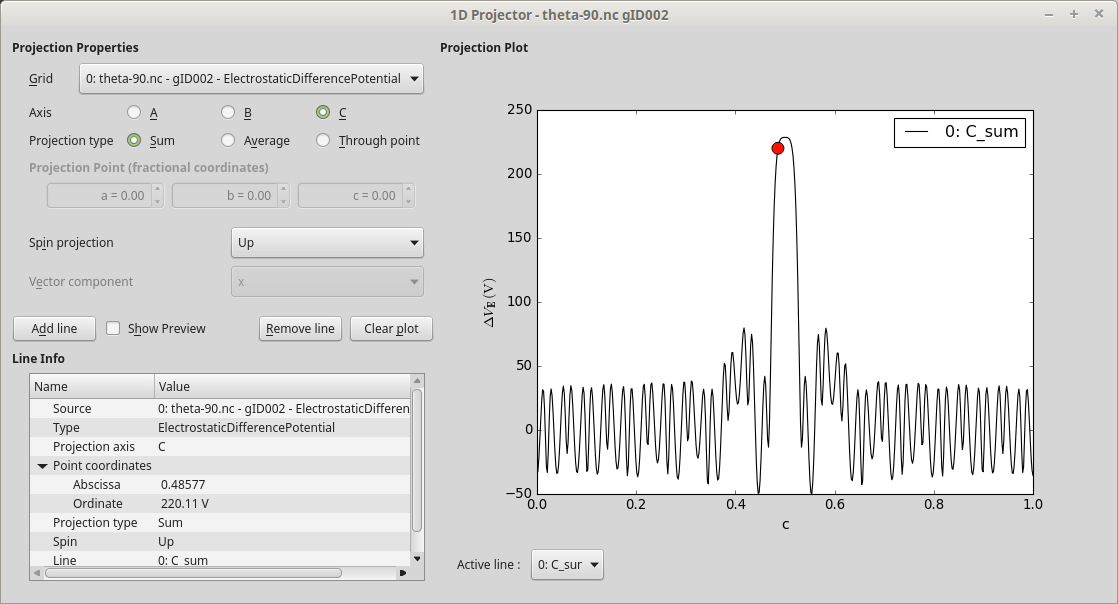
First of all, select the electrostatic difference potential and plot it using the 1D Projector in order to check that the NEGF calculation converged to a well-behaved ground state: Project the average EDP onto the C axis, and observe that the ground state electrostatic potential is nicely periodic in both ends of the device toward the electrodes, as it should be, and has the expected non-periodic feature around the gap in the middle of the device.
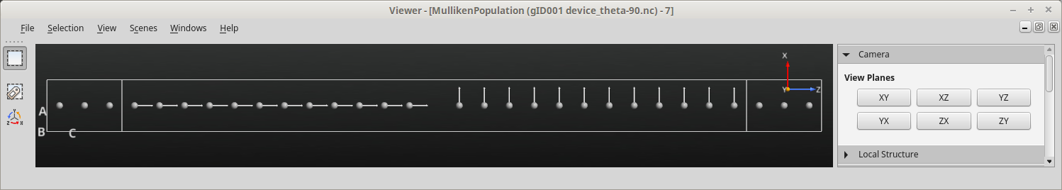
Next, select the Mulliken population analysis item and open it in the
 Viewer. Use the Camera options (or click
  )
to select the ZX plane for a clear view of the spin orientations.
)
to select the ZX plane for a clear view of the spin orientations.
Calculate the STT
You are now ready to use linear response (LR) theory to calculate the spin transfer
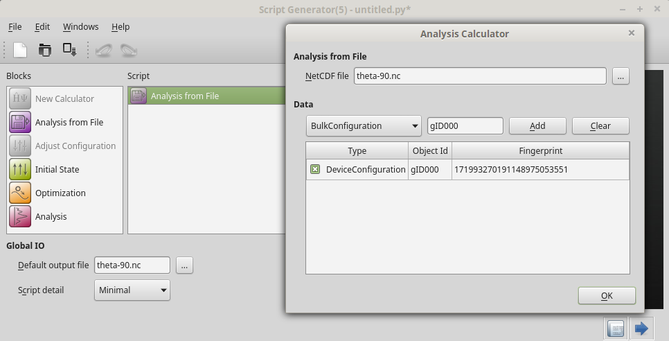
torque. Open a new Script Generator window
and add the  Analysis from File block. Open the block
and select the device configuration saved in
Analysis from File block. Open the block
and select the device configuration saved in theta-90.nc
for post-SCF analysis. Then change the Script Generator default output file
to theta-90.nc in order to save all calculated quantities in that file.
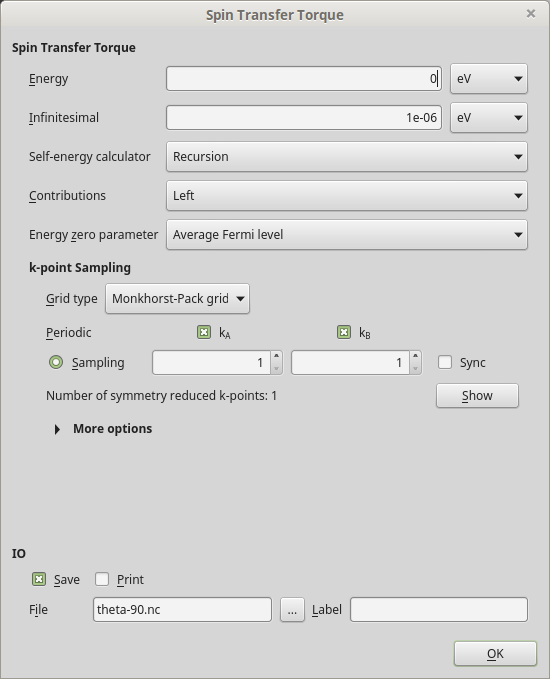
Add also the  analysis block, and open it to see the available options. Note in particular
3 important settings:
analysis block, and open it to see the available options. Note in particular
3 important settings:
- Energy:
The electron energy, with respect to the Fermi level, for which the STT will be calculated.
- Contributions:
The STT is by default calculated for the left –> right current.
- k-points:
Fairly dense k-point grids are sometimes needed along periodic directions orthogonal to the transport direction.
Tip
See the QuantumATK Manual entry SpinTransferTorque for a full description
of all input parameters for the STT calculation and all QuantumATK Python methods
available on the object.
Leave all the STT options at defaults and save the script as stt.py.
The script should look roughly like this: stt.py. Run the calculation
using the Job Manager – it should finish in less
than a minute.
The STT analysis object should now have been added to the file theta-90.nc
and be available on the QuantumATK LabFloor:
 SpinTransferTorque
Important
The spin transfer torque depends on the bias voltage across the electrodes, and is of course zero at zero bias, since no current flows. The linear-response spin transfer torque (LR-STT) assumes a linear relationship between the STT and the bias voltage \(V\),
where \(\tau\) is a linear-response coefficient. The QuantumATK SpinTransferTorque analysis object computes the local components of the LR-STT coefficient \(\tau\), from which the small-bias STT may be calculated.
Use first the Viewer to get a 3D visualization of the values
of the LR-STT coefficient for \(\theta\)=90°:
Open the Mulliken population in the Viewer,
and then drag-and-drop the STT item onto the Viewer window. The coefficient \(\tau\)
is represented on a 3D vector grid, each vector consisting of the local x-,
y-, and z-components, so you need to choose which component
to visualize. Choose in this case to visualize the y-component as an isosurface:

You can also use the 1D Projector to visualize the STT components. Select the STT item on the LabFloor, and click the 1D Projector plugin. Plot the x, y, and z vector components in the same plot, projected on the C axis.
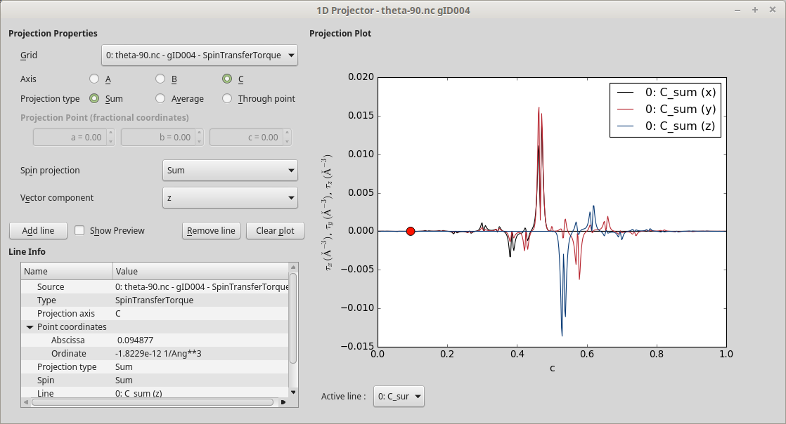
It is common to divide the STT into out-of-plane and in-plane contributions. In the present case, the magnetizations in the left and right electrodes point in the z- and x-directions, respectively, thus defining the in-plane contribution as being in the XZ-plane, while the y-component gives the out-of-plane contribution.
The two figures below show the out-of-plane and in-plane components of the LR-STT coefficient. The spin of the current is oriented along z when entering the right part of the device, and is then turned such as to be aligned along x. The x-component of \(\tau\) is therefore non-zero only in the left-hand part of the device, while the z-component is non-zero only in the right-hand part. The two components are in this case mirror images of each other.

Tip
Both figures above were generated using the 1D Projector. If you right-click the plot and select Customize, a dialog appears where you can customize plot details such as title, legend, colors, etc.
Angle Dependence
Let us next investigate how the LR-STT coefficient depends
on the angle \(\theta\) in the interval 0° to 180°.
What is needed is a range of range of zero-bias NEGF calculations for different
values of \(\theta\), each followed by calculation of the SpinTransferTorque
analysis object for that particular spin configuration. This is most easily
achieved by combining the main parts of the scripts theta-90.py and
stt.py used above:
 1thetas = [0,10,20,30,40,50,60,70,80,100,110,120,130,140,150,160,170,180]
 2
 3for theta in thetas:
 4    # Output data file
 5    filename = 'theta-%i.hdf5' % theta
 6
 7    # Read in the collinear calculation
 8    device_configuration = nlread('para.hdf5', DeviceConfiguration)[0]
 9
10    # Use the special noncollinear mixing scheme
11    iteration_control_parameters = IterationControlParameters(
12        algorithm=PulayMixer(noncollinear_mixing=True),
13    )
14
15    # Get the calculator and modify it for noncollinear LDA
16    calculator = device_configuration.calculator()
17    calculator = calculator(
18        exchange_correlation=NCLDA.PZ,
19        iteration_control_parameters=iteration_control_parameters,
20    )
21
22    # Define the spin rotation in polar coordinates
23    left_spins  = [(i, 1, 0*Degrees,    0*Degrees) for i in range(12)]
24    right_spins = [(i, 1, theta*Degrees, 0*Degrees) for i in range(12,24)]
25    spin_list   = left_spins + right_spins
26    initial_spin = InitialSpin(scaled_spins=spin_list)
27
28    # Setup the initial state as a rotated collinear state
29    device_configuration.setCalculator(
30        calculator,
31        initial_spin=initial_spin,
32        initial_state=device_configuration,
33    )
34
35    # Calculate and save
36    device_configuration.update()
37    nlsave(filename, device_configuration)
38
39    # -------------------------------------------------------------
40    # Mulliken Population
41    # -------------------------------------------------------------
42    mulliken_population = MullikenPopulation(device_configuration)
43    nlsave(filename, mulliken_population)
44    nlprint(mulliken_population)
45
46    # -------------------------------------------------------------
47    # Transmission Spectrum
48    # -------------------------------------------------------------
49    kpoint_grid = MonkhorstPackGrid(
50        force_timereversal=False
51    )
52
53    transmission_spectrum = TransmissionSpectrum(
54        configuration=device_configuration,
55        energies=numpy.linspace(-2,2,101)*eV,
56        kpoints=kpoint_grid,
57        energy_zero_parameter=AverageFermiLevel,
58        infinitesimal=1e-06*eV,
59        self_energy_calculator=RecursionSelfEnergy(),
60        )
61    nlsave(filename, transmission_spectrum)
62
63    # -------------------------------------------------------------
64    # Spin Transfer Torque
65    # -------------------------------------------------------------
66    kpoint_grid = MonkhorstPackGrid(
67        force_timereversal=False,
68        )
69
70    spin_transfer_torque = SpinTransferTorque(
71        configuration=device_configuration,
72        energy=0*eV,
73        kpoints=kpoint_grid,
74        contributions=Left,
75        energy_zero_parameter=AverageFermiLevel,
76        infinitesimal=1e-06*eV,
77        self_energy_calculator=RecursionSelfEnergy(),
78        )
79    nlsave(filename, spin_transfer_torque)
The Mulliken population and transmission spectrum are not strictly needed, but will prove useful for further analysis later on. Notice that the case \(\theta\)=90° is skipped because that calculation was already done above.
Download the script, angles.py, and run it using the
Job Manager – it may take up to 30 minutes to complete.
When the job finishes you have a number of new nc-files on the QuantumATK LabFloor, each for a particular spin angle. You may visualize the Mulliken populations to check for yourself that the spin angle varies correctly.
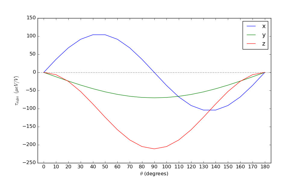
Use the script angles_plot.py to analyze and plot the results. For each angle,
it sums the x-, y- and z-components of \(\tau\) in the
right-hand part of the device, and plots them against the angle:
 1# Prepare lists
 2thetas = [0,10,20,30,40,50,60,70,80,90,100,110,120,130,140,150,160,170,180]
 3x = []
 4y = []
 5z = []
 6
 7# Read data
 8for theta in thetas:
 9    # Data file
10    filename = 'theta-%i.hdf5' % theta
11
12    # Read in the STT analysis object
13    stt = nlread(filename, SpinTransferTorque)[0]
14
15    # Get the STT 3D vector grid (units Bohr**-3)
16    array = stt.toArray()
17
18    # Get the index of middle position along C
19    sh = numpy.shape(array)
20    k = sh[2]/2
21
22    # Get the volume element of the STT grid.
23    dX, dY, dZ = stt.volumeElement()
24    volume = numpy.abs(numpy.dot(dX, numpy.cross(dY, dZ)))
25
26    # Integrate the vector components in the right-hand part of the device
27    stt_x = numpy.sum(array[:,:,k:,:,0])*volume*stt.unit()
28    stt_y = numpy.sum(array[:,:,k:,:,1])*volume*stt.unit()
29    stt_z = numpy.sum(array[:,:,k:,:,2])*volume*stt.unit()
30
31    # append to lists
32    x.append(stt_x)
33    y.append(stt_y)
34    z.append(stt_z)
35
36# Convert lists to arrays
37x = numpy.array(x)
38y = numpy.array(y)
39z = numpy.array(z)
40
41# Save data for future convenience
42import pickle
43f = open('angles_plot.pckl', 'wb')
44pickle.dump((thetas,x,y,z), f)
45f.close()
46
47# Plot results
48import pylab
49pylab.figure(figsize=(10,6))
50pylab.plot(thetas, x*1e6, label='x')
51pylab.plot(thetas, y*1e6, label='y')
52pylab.plot(thetas, z*1e6, label='z')
53pylab.axhline(0, color='k', linestyle=':')
54pylab.legend()
55pylab.xlabel(r'$\theta$ (degrees)')
56pylab.ylabel(r'$\tau_\mathrm{right} \, \, \, (\mu eV/V)$')
57ax = pylab.gca()
58ax.set_xlim((-5,185))
59ax.set_xticks(thetas)
60pylab.savefig('angles_plot.png')
61pylab.show()
The in-plane STT may also be compared to an analytic expression from Ref. [1]:
where \(T_z(180^\circ)=h/(4\pi e)[T_\uparrow(180^\circ)-T_\downarrow(180^\circ)]\) is the spin transmission for the anti-parallel configuration, and likewise for \(T_z(0^\circ)\). The vector \(\mathbf{M}_{L/R}\) is the direction of magnetization in the left/right part of the carbon chain.
Use the script analytical.py to do the analysis. It computes the
in-plane (\(\tau_\parallel = \sqrt{\tau_x^2 + \tau_z^2}\))
and out-of-plane (\(\tau_\perp = \tau_y\))
components in the right-hand part of the device,
and also computes \(\tau_\parallel\) from the analytical expression
using the obtained transmission spectrum at each angle:
 1# Load STT data
 2import pickle
 3f = open('angles_plot.pckl', 'rb')
 4(thetas,x,y,z) = pickle.load(f)
 5f.close()
 6
 7# Process STT data
 8inplane = (x**2 + z**2)**0.5
 9outplane = y
10
11# Analytical in-plane STT
12transmissions = numpy.zeros(2)
13for j,theta in enumerate([0,180]):
14    # Data file
15    filename = 'theta-%i.hdf5' % theta
16    # Read the transmission spectrum
17    transmission = nlread(filename, TransmissionSpectrum)[0]
18    # Get the energies
19    energies = transmission.energies().inUnitsOf(eV)
20    # Find the index of the Fermi level
21    i_Ef = numpy.argmin(abs(energies))
22    # Calculate the spin-transmission (Up - Down)
23    T = transmission.evaluate(spin=Spin.Up)[i_Ef]-transmission.evaluate(spin=Spin.Down)[i_Ef]
24    # Append to list
25    transmissions[j] = T
26analytical = abs(transmissions[0]-transmissions[1])/2*numpy.sin(numpy.array(thetas)*numpy.pi/180)/(2*numpy.pi)
27
28# Plot results
29import pylab
30pylab.figure(figsize=(10,6))
31pylab.plot(thetas, inplane*1e6,         label=r'$\tau_\parallel$')
32pylab.plot(thetas, analytical*1e6, 'o', label=r'$\tau_\parallel$'+'(analytical)')
33pylab.plot(thetas, outplane*1e6,        label=r'$\tau_\perp$')
34pylab.axhline(0, color='k', linestyle=':')
35pylab.legend()
36pylab.xlabel(r'$\theta$ (degrees)')
37pylab.ylabel(r'$\tau_\mathrm{right} \, \, \, (\mu eV/V)$')
38ax = pylab.gca()
39ax.set_xlim((-5,185))
40ax.set_xticks(thetas)
41pylab.savefig('analytical.png')
42pylab.show()
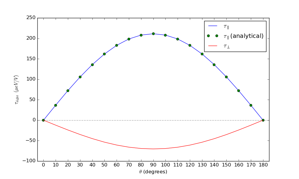
The agreement between the angle-dependent calculation (blue line) and the analytical results (green dots), obtained only from the spin transmissions in the parallel and anti-parallel configurations, is excellent.