Young’s modulus of a CNT with a defect
Carbon nanotubes are well known for their exceptional mechanical properties; Young’s moduli in the 1 TPa range have been measured [1], which is higher than any other known material. The theoretical Young’s modulus is fairly simple to calculate for a defect-free carbon nanotube, but this is not the case when defects are present. In that case, molecular dynamics (MD) is a suitable tool for calculation of the mechanical properties.
In this tutorial you will build a carbon nanotube (CNT) with a Stone–Wales defect, and use the ATK-ForceField engine to calculate the Young’s modulus.
Important
This tutorial uses a CNT structure that is built in the tutorial
Stone–Wales Defects in Nanotubes. If you have not already done so, please go that
tutorial first and build the CNT device configuration, or simply
download it as a Python script:
stone_wales_cnt.py.
CNT bulk configuration
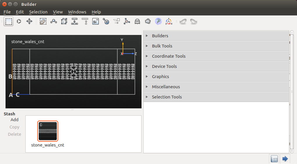
Open the QuantumATK Builder  , and use
to import the previously
saved CNT configuration to the Stash. Note that the structure is a
device configuration with the Stone–Wales defect in the middle of the central
region.
, and use
to import the previously
saved CNT configuration to the Stash. Note that the structure is a
device configuration with the Stone–Wales defect in the middle of the central
region.
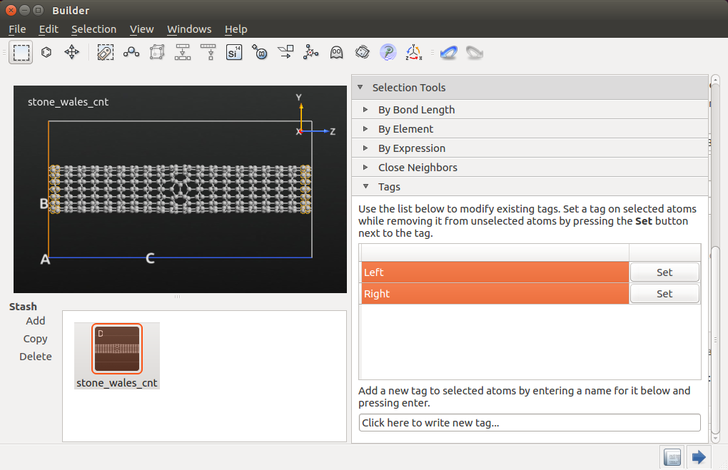
Next, highlight the device Stash item, and click the  icon to convert it to a bulk configuration (the device electrodes are
simply removed), and use the
tool to add tags to the atoms at both ends of the nanotube:
icon to convert it to a bulk configuration (the device electrodes are
simply removed), and use the
tool to add tags to the atoms at both ends of the nanotube:
Use the mouse to highlight the left-most carbon atoms and set the tag “Left” on them.
Do the same for the right-most carbon atoms, as illustrated below.
These tags will be used to impose constraints on the structure during the MD simulation.
Configuring the MD simulation
Send the CNT bulk configuration with the Stone–Wales defect to the Script Generator
 and add the
  New Calculator and
 blocks. Then edit both blocks to configure the calculation:
First, change the default output file to
mdtrajectory_cnt.hdf5.In the New Calculation block, select the ATK-ForceField calculator, and make sure to use the Tersoff_C_2010 classical potential, which is designed for simulating lattice dynamics of graphene and nanotubes.
Note
For QuantumATK-versions older than 2017, the ATK-ForceField calculator can be found under the name ATK-Classical.
Make the following changes to the MolecularDynamics block:
Molecular Dynamics options:
Set the “Type” to NVT Berendsen.
Set “Steps” to 20000.
Set the “Log interval” to 200.
Initial Velocity options:
Set “Type” to Maxwell-Boltzmann.
Set “Temperature” to 300 K.
Untick the Remove center-of-mass momentum option.
NVT Berendsen options:
Set the “Thermal coupling” to 1 fs.
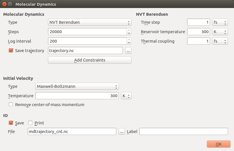
Leave the remaining settings at defaults, like in the image above.
Save the script as mdtrajectory_cnt.py and send it to the Editor
 by using the
  icon.
icon.
Adding Python hooks
It is possible in QuantumATK to define “hooks”; Python functions or classes that are called before or after each MD step. These hooks can be used to provide customized on-the-fly analysis or monitoring of the system, or – as in this case – to modify the structure dynamically during the simulation.
You will now define a pre-step hook that will be used to strain the nanotube slightly for each step of the MD run:
With the Python script open in the Editor, scroll down to the bottom of the script and locate the block defining the
md_trajectory. The predefined tags “Left” and “Right” can now be used to apply constraints to the system. Change the lineconstraints=[]
to
constraints=bulk_configuration.indicesFromTags(["Left","Right"])
In the
md_trajectoryblock, add the linespre_step_hook=strainer, write_stresses=True,
and add a comma to the line immediately above it (
method=method,). The first line will invoke the strainer hook function (defined below), and the second line will ensure that stresses are calculated and stored in the trajectory.You should also define what “strainer” is: Add the following line immediately before the
md_trajectoryblock:strainer = StressStrainUtility()
The bottom of the script should now look like this:
 1# -------------------------------------------------------------
 2# Molecular Dynamics
 3# -------------------------------------------------------------
 4
 5initial_velocity = MaxwellBoltzmannDistribution(
 6    temperature=300.0*Kelvin,
 7    remove_center_of_mass_momentum=False
 8)
 9
10method = NVTBerendsen(
11    time_step=1*femtoSecond,
12    reservoir_temperature=300*Kelvin,
13    thermostat_timescale=100*femtoSecond,
14    initial_velocity=initial_velocity
15)
16
17strainer = StressStrainUtility()
18
19md_trajectory = MolecularDynamics(
20    bulk_configuration,
21    constraints=bulk_configuration.indicesFromTags(["Left","Right"]),
22    trajectory_filename='mdtrajectory_cnt.hdf5',
23    steps=20000,
24    log_interval=200,
25    method=method,
26    pre_step_hook=strainer,
27    write_stresses=True
28)
Line 17 above initializes an instance of the class
StressStrainUtility, which is a Python class that you now will define. Insert the following at the very top of the script:1# Define a prestep function which can expand the system 2 3class StressStrainUtility: 4 """ Perform a strain of a configuration over time. """ 5 def __init__(self, delta=0.0001, skip=0): 6 """ 7 @param delta The strain to apply in each step 8 @param first steps to "skip" strain 9 """ 10 self.__delta = [0.0,0.0,delta]*Angstrom 11 self.__skip = skip 12 self.stresses = [] 13 self.lengths = [] 14 15 def __call__(self, step, time, configuration, forces, stress): 16 """ 17 Strainer call. 18 """ 19 # Get the lattice vectors. 20 u1, u2, u3 = configuration.primitiveVectors() 21 22 # Don't apply strain in the earliest MD steps 23 if step < self.__skip: 24 return 25 26 # Store the history 27 self.stresses.append( stress[2,2].inUnitsOf(eV/Angstrom**3) ) 28 self.lengths.append( u3[2].inUnitsOf(Angstrom) ) 29 30 # Increase the lattice vectors. 31 u3 = u3 + self.__delta 32 33 # Set the new lattice. 34 configuration.setBravaisLattice(UnitCell(u1,u2,u3)) 35 36 # Move all the atoms that are constrained on the right side. 37 constraints = configuration.indicesFromTags("Right") 38 for c in constraints: 39 xyz = numpy.array(configuration.cartesianCoordinates()[c]) + numpy.array(self.__delta) 40 configuration.setCartesianCoordinates(indices=[c], cartesian_coordinates=[xyz]*Angstrom) 41 42 def length(self): 43 return numpy.array(self.lengths)*Angstrom 44 45 def stress(self): 46 return numpy.array(self.stresses)*eV/Angstrom**3 47
This class defines a method to enable straining of a unit cell along the z-direction. You will use it to study how a CNT with a defect responds to strain.
As you can see from the script, the class has two inputs, delta and skip:
- delta
defines how much the u3 vector (the z-direction) is expanded on every step in the MD calculation.
- skip
defines how many steps should pass before the configuration will be strained.
The actual straining is done in the “for-loop” beginning at line 38,
by increasing the coordinates of the atoms tagged “Right” by the amount delta
along the z-direction. On lines 27 and 28, the stress and total length of the
configuration are calculated and appended to two separate lists. These will be
used later for plotting.
Tip
By writing pre_strain_hook=strainer in the md_trajectory block,
the class (technically, the method __call__) is called before the force and energy
calculation in every MD step (for more details about hook functions see
MolecularDynamics()).
Computing Young’s modulus
To properly calculate the Young’s modulus, it is necessary to take the total volume of the simulation domain into account. The stress reported by QuantumATK therefore has to be multiplied by the total volume of the cell and then divided by the volume of the nanotube.
Several definitions of the volume of a CNT. A common
way of defining it is to say that the wall of the nanotube extends for
half a \(\pi\)-bond in and out of the wall, so that it becomes a
cylindrical shell with thickness equal to that of a \(\pi\)-bond,
approximately 1.35 Å, so that the total cross-sectional area is 1.35 Å
times the circumference of the nanotube. The circumference for a
(5,5)-armchair nanotube is
\(5 \times (3 \times x)\), where \(x\)=1.42 Å is the carbon-carbon
bond length. Finally, for the volume, you need the length of the tube,
which is given in the .hdf5 file saved by QuantumATK.
At the bottom of the script, delete the line
nlsave('mdtrajectory_cnt.hdf5', md_trajectory).Add instead the following lines of code in order to invoke the proper stress calculation:
# -------------------------------------------------------------
# Finding Young's Modulus
# -------------------------------------------------------------

# Find center of cnt from mean x- and y-coordinates
coords = bulk_configuration.cartesianCoordinates()
x_coords = coords[:,0]
y_coords = coords[:,1]
x_0 = numpy.sum(x_coords)/len(x_coords)
y_0 = numpy.sum(y_coords)/len(y_coords)

# Find radius by mean distance from center to atoms' x- and y-coordinates
radius = numpy.sum( ( (x_coords - x_0)**2 + (y_coords - y_0)**2 )**(1/2.0) ) / len(x_coords)

# Find cross-sectional area by multiplying circumference with length of a pi-bond
pi_bond = 1.35
circumference = radius * 2 * numpy.pi
area = circumference * pi_bond

# Find volumes of CNT and of whole cell
volume_cnt = area * strainer.lengths[-1]

u1, u2, u3 = bulk_configuration.bravaisLattice().primitiveVectors()
volume_cell = u1[0] * u2[1] * u3[2]

# Factor the stresses to the volume of the CNT
stresses_factored = numpy.array(strainer.stresses * (volume_cell / volume_cnt) )*eV/Angstrom**3

# Calculate the strain
strain = (strainer.length() - strainer.length()[0] ) / strainer.length()[0]

# Calculate Young's modulus in TPa
modulus = (stresses_factored[-1].inUnitsOf(Pa) - stresses_factored[0].inUnitsOf(Pa) ) / float(strain[-1]) / 1e12
print("Young's Modulus: {} TPa".format(modulus))
Finally, add a few lines of code that will save different parts of the calculation and plot the results using pylab.
# Save the result to a file.
print(strainer.length())
nlsave("mdtrajectory_cnt.hdf5", md_trajectory, "MD")
nlsave("mdtrajectory_cnt.hdf5",strainer.length(), "C length")
nlsave("mdtrajectory_cnt.hdf5",strainer.stress(), "C stress")
nlsave("mdtrajectory_cnt.hdf5",stresses_factored, "C stresses factored")

# Plot stress-strain curve.
import pylab
pylab.figure()
pylab.plot(strain * 100, stresses_factored.inUnitsOf(GPa))
pylab.title('CNT with Stone-Wales defect')
pylab.xlabel('Strain (%)')
pylab.ylabel('Stress (GPa)')
pylab.grid(True)
pylab.savefig("mdtrajectory_cnt_fig.png")
The script is now ready to be executed. You may download the script to
make sure you did the manual editing correctly:
mdtrajectory_cnt.py.
Send the script to the Job Manager  by clicking
the icon, then save it, and run it. The job should take
around 3 minutes on a laptop.
by clicking
the icon, then save it, and run it. The job should take
around 3 minutes on a laptop.
Visualize and analyse the results
The nanotube lengths and stresses that occur during the MD simulation run
are saved in the .hdf5 file with different ID’s (“C length”, “C stress”,
and “C stresses factored”). These are used to produce the plot titled
mdtrajectory_cnt_fig.png, which is automatically saved in the
project folder. It shows the stress vs. strain relationship for the nanotube,
which is also shown below. The linear (elastic) behavior for small strains
make it possible to calculate Young’s modulus E for the nanotube,
defined as E = stress/strain.
With this procedure, the calculated Young’s modulus of the carbon nanotube with one Stone–Wales defect is around 2.3 TPa (it may vary across different MD runs). This is pretty far from the calculated value of 1.28 TPa for defect-free nanotubes [2]. However, as shown in [1], nanotubes with defects have in general a higher Young’s modulus.
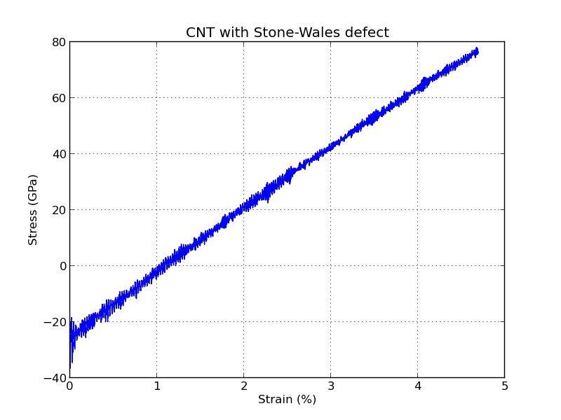
Note
The figure above shows that the stress is negative for small stress levels, which means that the nanotube is actually under compressive stress until around 1.1% strain.
This could be avoided by running a geometry optimization step before running the MD calculation, which can be done using the Optimization block available in the Script Generator. However, for the strains investigated here, the CNT shows a linear stress–strain behavior, so the obtained Young’s modulus should not change significantly if a geometry optimization is performed first.
The data file mdtrajectory_cnt.hdf5 should be shown on the LabFloor.
Select the file and click the Movie Tool in the right-hand plugins panel.
The Movie Tool can be used to inspect MD trajectories; it will show a movie of
the simulation and data about energies and temperatures. The tool looks like
illustrated below.
Tip
Right click the mouse and select Show bonds to visualize the bond connection between the carbon atoms.
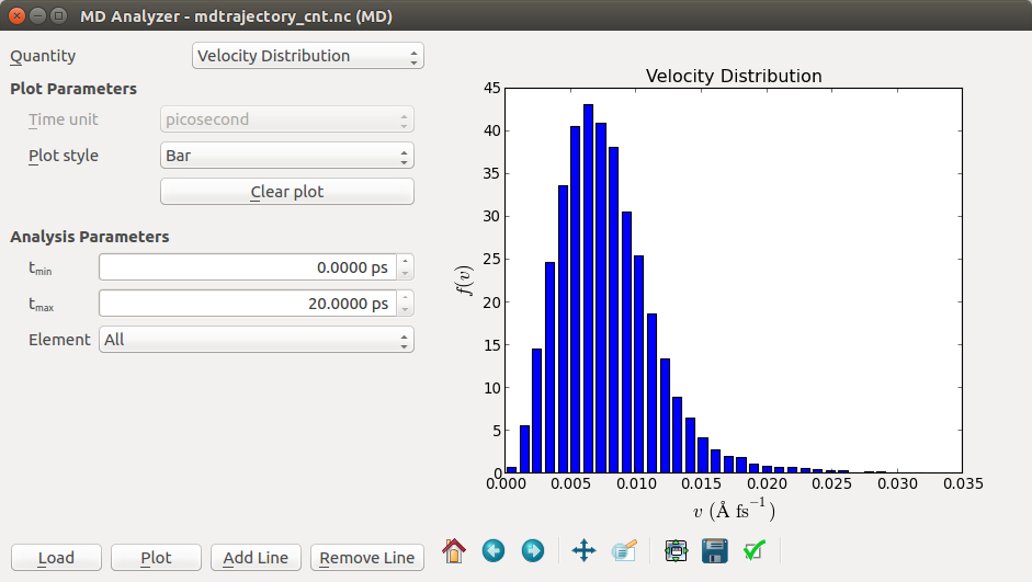
Another useful plugin is the MD Analyzer, which can show the radial distribution, velocity distribution, and the kinetic energy distribution of the atoms in the system. A screenshot of the velocity distribution is shown below.