The DFTB model in ATK-SE
The purpose of this tutorial is to show you how to install new parameter sets into the Density Functional based Tight Binding (DFTB) model [1], [2] implemented in ATK-SE.
ATK is shipped with Slater-Koster parameter files from the CP2K and Hotbit consortia, for use in the semi-empirical DFTB model. This tutorial will show how to download additional parameters from the DFTB website and install them such that they work as a native part of ATK.
Once the parameters are installed, they can be used for modeling molecules, bulk and device systems. In this tutorial, you will first download and install a DFTB parameter set, and then learn how to calculate properties of spin polarized bulk systems using a Slater-Koster calculator.
Note
You will primarily use the graphical user interface QuantumATK for setting up and analyzing the results. If you are not familiar with QuantumATK, we recommend you first go through a few of the QuantumATK Tutorials.
The underlying calculation engine for this tutorial is ATK-SE, the semi-empirical part of QuantumATK. A complete description of all the parameters, and in many cases a longer discussion of their physical relevance, can be found in the ATK Reference Manual.
In order to run this tutorial, and in general use the semi-empirical models in ATK, you must have a license for ATK-SE. If you do not have one, you may obtain a time-limited demo license by contacting us via our website: Contact QuantumATK.
Installing DFTB parameters
Getting a DFTB license
The dftb.org website has a number of parameters for the DFTB method, which can be used with ATK-SE. In order to download the parameters, you will need to fill out their registration form. When your registration has been processed, you will receive a username and password to their website.
Downloading the parameters
On the DFTB download page, you can get an overview of the different DFTB parameter sets. The primary ones are named “mio”, “pbc”, and “matsci”; the “mio” set can further be extended by a number of specialized sets listed further below. The page also lists the papers that must be referenced when using the parameter sets.
Log into dftb.org and download the parameter sets of your interest.
The downloaded files will be in a compressed tar ball (.tar.gz).
Installing the parameters
ATK has a special folder for each of the three DFTB parameters sets.
For instance, to install the “mio” parameter set, unpack the downloaded tar ball
and copy the .skf files to the directory share/tightbinding/dftb/mio/
in the directory where ATK is installed.
In Linux you can use the following commands:
tar zxvf mio-1-1.tar.gz
cp mio-1-1/* [ATKPATH]/share/tightbinding/dftb/mio
where [ATKPATH] is the path to your installation of QuantumATK.
Similarly, the “pbc” and “matsci” parameter files should be copied to the dftb/pbc and dftb/matsci directories.
Note that these directories already exist, but are empty.
Warning
If you use QuantumATK on a laptop or workstation to set up the calculations, and then a separate installation of ATK on a cluster for running the calculations, then the parameter files must be installed on both systems separately.
Testing the installation
Bandstructure calculation
To test that the parameters are correctly installed you, can perform the following bandstructure calculation for graphene.
Start QuantumATK and create a new project, then click Open.
Launch the
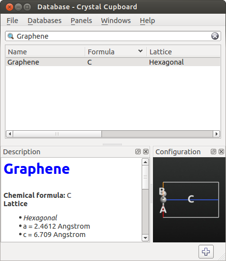
 Builder and click . Find Graphene.
Add the structure to the Stash (double-click or use the
 icon).
Send the structure to the
 Script Generator using the
  button.
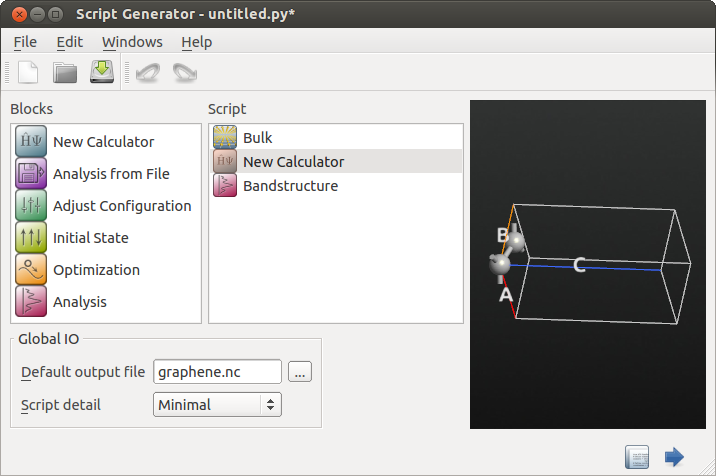
In the Script Generator, add the following blocks:
 New Calculator
 Bandstructure
Change the output filename to
graphene.nc.
The Script Generator should now have the following settings:
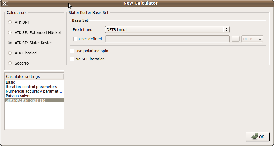
Now open the New Calculator block and make the following changes:
Select the ATK-SE: Slater-Koster calculator.
Change the k-point sampling to (5, 5, 1).
Go to the Slater-Koster basis set, and check that the installed basis sets are in the basis set list. Select the “DFTB [mio]” basis set.
Note
If you do not see the “DFTB [mio]” basis set in the list, something went wrong in the installation process.
Check that the file atkpython/share/tightbinding/dftb/mio/C-C.skf exists in your ATK installation directory.
Uncheck the No SCF iteration box, in order to invoke a self-consistent DFTB calculation.
Attention
The default assumption is that a tight-binding model is non-self-consistent. It is the responsibility of the user to uncheck the No SCF iteration box for models which are to be self-consistent. Most DFTB models are self-consistent.
Transfer the script to the
 Job Manager using the Send To button (), and start the calculation.
When the job has finished, locate the file
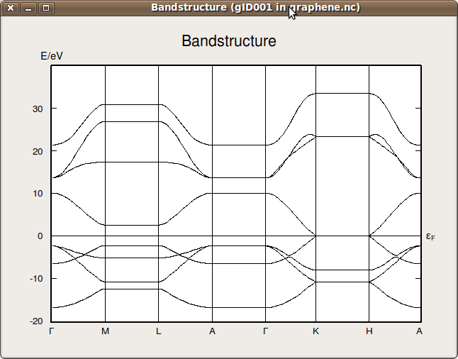
graphene.ncunder project files in the main QuantumATK window, and plot the bandstructure using the Bandstructure Analyzer from the right-hand tool bar. You should get the result shown below:
Note
If the test went well, the DFTB parameters are properly installed. You are then able to use DFTB parameters instead of DFT for some of the other ATK tutorials available on the QuantumATK website (including quantum transport calculations), in order to save computational time.
Obviously, this only works if the elements used are covered by the DFTB basis sets.
Spin polarized calculations with DFTB
Calculating the spin polarization of a graphene ribbon
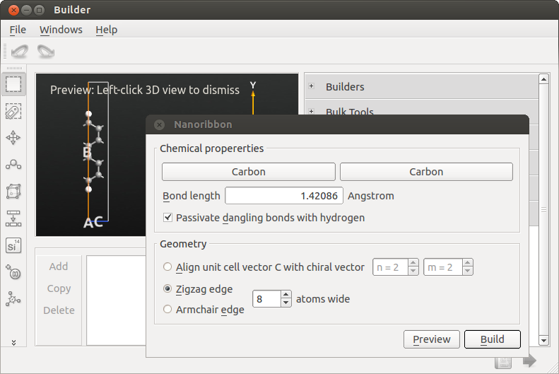
In the following you will set up a graphene nanoribbon, and perform a spin-polarized calculation using the DFTB [mio] model.
Open the
Builder and click .Build a zigzag ribbon that is 8 atoms wide.
To set up a calculation of the band structure,
send the structure to the Script Generator
using the button in the lower right-hand corner of the builder window.
In the Script Generator, add the following blocks:
- New Calculator
 Initial State
- Bandstructure
and change the output filename to ribbon.nc.
The Script Generator should now have the following settings:

Open the New Calculator block.
Select the ATK-SE: Slater-Koster calculator.
Change the k-point sampling to (1,1,11).
Go to the Slater-Koster basis set and select the “DFTB [mio]” basis set.
Check the Use polarized spin box, in order to perform a spin-polarized DFTB calculation.
Note
The DFTB parameter set does not include spin polarization parameters. Instead, spin polarization parameters are obtained from the ATK_W database.
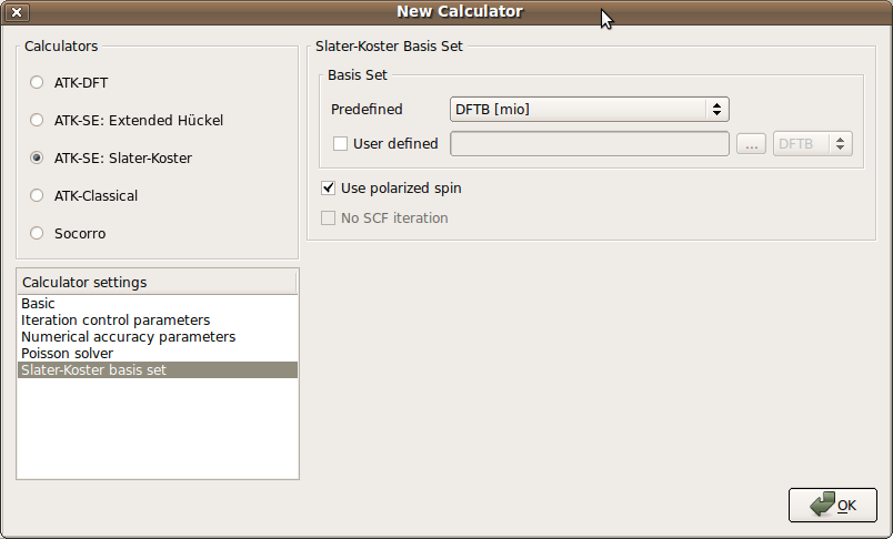
Finish by clicking OK.
Next, set up the initial spin state of the system:
Open the
Initial State block by double-clicking it.Set the Initial state type to User spin.
Under Spin, set the default spin of both Carbon and Hydrogen to 0.
- In the 3D view:
Click the upper carbon atom (index 0 in the list of atoms) and set its initial relative spin to 1.0.
Repeat this procedure for the lower carbon atom (number 1 in the list), setting its initial relative spins to -1.0. (Don’t be confused by the fact that the carbon atoms are not ordered by Y coordinate).
Leave the hydrogen atoms and the other carbon atoms with initial relative spin values of 0.0.
The dialogue should now look as shown below.

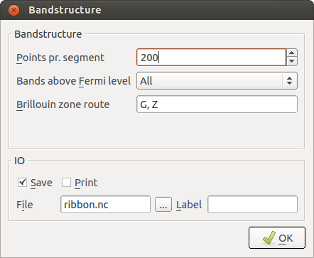
Finally, open the Bandstructure block:
Change Points pr. segment to 200. This implies that each band will be calculated with a resolution of 200 points.
Also notice that the default suggested route in the Brillouin zone (from the \(\Gamma\)-point G=(0,0,0) to Z=(0,0,1/2) in units of the reciprocal lattice vectors) is the appropriate one.
Send the script to the
Job Manager and run it.Return to the main QuantumATK window and select the file
ribbon.ncand plot the bandstructure.By using the zoom functionality, you should be able to obtain the following figure:

Calculate the properties of a series of configurations using scripting
If you want to calculate the bandstructure of a number of nanoribbons, it is very convenient to use Python scripting. The script below performs a calculation of the bandstructure of nanoribbons with chiral index (n,n), where n runs from 1 to 10.
Attention
The chiral index notation for nanoribbons in ATK is based on the linear combination of the planar graphene unit vectors that are used to form the unit cell. Thus, (n,n) have zigzag edges, and actually correspond to an unrolled armchair nanotube with the same chiral indices.
For armchair edge nanoribbons, the chiral indices are (n,0).
# Setup the DFTB Calculator
basis_set = DFTBDirectory("dftb/mio/")
pair_potentials = DFTBDirectory("dftb/mio/")

numerical_accuracy_parameters = NumericalAccuracyParameters(
    k_point_sampling=(1, 1, 51),
    )

iteration_control_parameters = IterationControlParameters()

calculator = SlaterKosterCalculator(
    basis_set=basis_set,
    pair_potentials=pair_potentials,
    numerical_accuracy_parameters=numerical_accuracy_parameters,
    iteration_control_parameters=iteration_control_parameters,
    spin_polarization=True,
    )

#loop over different NanoRibbons
for n in range(1,10):
    #generate the nanoribbon
    bulk_configuration = NanoRibbon(n,n)

    #Determine the initial spin of the configuration
    elements = bulk_configuration.elements()
    coords = bulk_configuration.fractionalCoordinates()
    scaled_spins = numpy.zeros(len(elements))

    #find the index of the two edge Carbon atoms,
    ymin = 0.5
    ymax = 0.5
    imin=0
    imax=0
    for i in range(len(elements)):
        if coords[i][1] < ymin and elements[i] == Carbon:
            ymin = coords[i][1]
            imin = i
        if coords[i][1] > ymax and elements[i] == Carbon:
            ymax = coords[i][1]
            imax = i

    # set opposite spins on the edge Carbon atoms
    scaled_spins[imin] = 1
    scaled_spins[imax] = -1

    #attach calculator, and set the initial spin
    bulk_configuration.setCalculator(
        calculator(),
        initial_spin=InitialSpin(scaled_spins=scaled_spins),
        )
    bulk_configuration.update()

    # Calculate Bandstructure
    bandstructure = Bandstructure(
        configuration=bulk_configuration,
        route=['G', 'Z'],
        points_per_segment=200,
        bands_above_fermi_level=All
    )
    nlsave('bandgap.nc',bandstructure)
Download the script to the project folder (
bandgap.py) and send it to the Job Manager by drag-and-drop in the QuantumATK window.This will generate the file
bandgap.nc.To analyze the data, download (
analyze_bandgap.py) and drop the following script on the Job Manager.
w_list = []
gap0_list = []
gap1_list = []
# read a list with the bandstructure data
bandstructure = nlread('bandgap.hdf5', Bandstructure)

for i in range(len(bandstructure)):
    # get all the bandlines
    energies = bandstructure[i].evaluate().inUnitsOf(eV)
    #calculate the number of occupied bands
    occupied_bands = numpy.sum(numpy.array(energies[0]) < 0)
    #calculate the minimum direct band gap
    gap0 = numpy.min(energies[:,occupied_bands]- energies[:,occupied_bands-1])
    #calculate the band gap at the zone boundary
    gap1 = energies[-1,occupied_bands]- energies[-1,occupied_bands-1]
    #determine the coordinates in the y direction
    y_values = NanoRibbon(i+1,i+1).cartesianCoordinates().inUnitsOf(Ang)[:,1]
    # calculate the width, as distance between furthest carbon atoms
    # i.e. calculate the  H-H distance and subtracting the C-H distance
    w = numpy.max(y_values)-numpy.min(y_values)-2.2
    #append calculated values to the list
    w_list.append(w)
    gap0_list.append(gap0)
    gap1_list.append(gap1)

#print the data
import pylab
pylab.figure()
pylab.plot(w_list,gap0_list, 'k-o')
pylab.plot(w_list,gap1_list, 'k-o', markerfacecolor='white')
pylab.xlabel(r"$w_z$ ($\AA$)", size=16)
pylab.ylabel("$\Delta_z$ (eV)", size=16)
pylab.show()
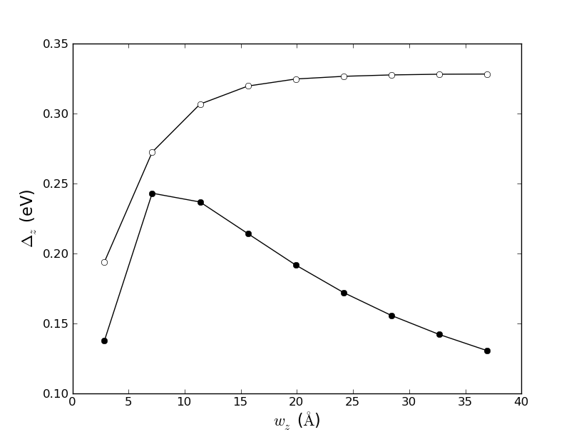
Fig. 126 Direct band gap (solid circles) and the band gap at the zone boundary as function of the width of the nanoribbon.
Attention
Except for the smallest ribbon, the plot shows the same qualitative behavior as Fig. 4c in Ref. [3]. The discrepancy in the results are related to the accuracy of the DFTB method compared with a DFT-LDA calculation. To test this, you can modify the script and change the definition of the calculator:
calculator = LCAOCalculator(
    numerical_accuracy_parameters=numerical_accuracy_parameters,
    exchange_correlation = LSDA.PZ
    )
Remember to also modify the name of the output file in order to separate the new data from the old data. Then execute the script.
References