Hybrid Functionals
Hybrid functionals are exchange-correlation functionals that take into account exact Fock exchange
[1]. There are different approaches as to how to mix in the exact exchange. The
method we implemented in our PlaneWaveCalculator code is the HSE functional described in
[2][3].
Background
The HSE functional is an adaptation of the PBE0 functional [4], where the exchange-correlation energy is defined as:
The exact-exchange energy \(E^\text{HF}_x\) is defined in terms of the Kohn-Sham orbitals as:
and is very expensive to evaluate.
For periodic systems, the exact-exchange energy converges very slowly with the distance. For this reason Heyd et al. [2] suggested splitting up the exchange in a long- and short-range part (defined by a screening length parameter \(\mu\)). In which only for the short range part exact exchange is mixed:
The most general version of this functional depends on two parameters, the screening length \(\mu\), and the mixing fraction \(\alpha\), which was \(\frac{1}{4}\) in the PBE0 functional:
ACE Implementation
To include the exact exchange energy in the total energy functional in a DFT calculation one needs to add a non-local orbital dependent exact exchange potential, \(V^\text{HF}_x [\psi_{\mathbf{k}n}(\mathbf{r})] = \frac{\delta E^\text{HF}_x}{\delta \psi_{\mathbf{k} n}^*(\mathbf{r})}\) to the Hamiltonian when solving the Kohn-Sham equations. Even though only action of the exchange potential operator is needed when iteratively solving for eigensolutions, the evaluation of the operator is still very expensive compared to the other parts of a DFT calculation, and it has to be carried out several times in the iterative process.
However, using the Adaptively Compressed Exchange operator method [5] we avoid the expensive re-evaluations of the exchange operator in the subsequent steps in the iterative eigensolver. In this approach the exact-exchange operator \(\hat{V}^{\text{HF}}_x\) is applied once to the current best estimate for the ground state wave-functions, \(|\psi_i\rangle\),
From these \(W\) states, a set of so-called ACE projectors \(|p_i\rangle\) are constructed. The projection operator:
has the same action as \(\hat{V}^\text{HF}_x\) on states in the subspace spanned by the wave functions and can be proven to a good approximation for states that are close to the subspace. The advantage is that \(\hat{V}^\text{ACE}_x\) is much cheaper to apply (same computational complexity as the pseudopotential) in the following uses of the Hamiltonian. Note, however, that to construct the ACE projectors, one needs to fully evaluate the action of the full exact exchange operator, \(\hat{V}^\text{HF}_x\), a process which is still very expensive and scales as
where \(N_\tilde{\mathbf{k}}\) is the number of symmetry-reduced \(\mathbf{k}\)-points, \(N_\mathbf{k}\) is total number of unreduced \(\mathbf{k}\)- points, \(N_\text{band}\) is the number of occupied bands and \(N_\mathbf{G}\) is the number of plane wave basis functions.
Instead of only using the ACE operator for a single SCF iteration it has proven more efficient to keep the operator fixed and do a full self-consistent cycle before updating the ACE projectors from the most recent Kohn-Sham wave functions.
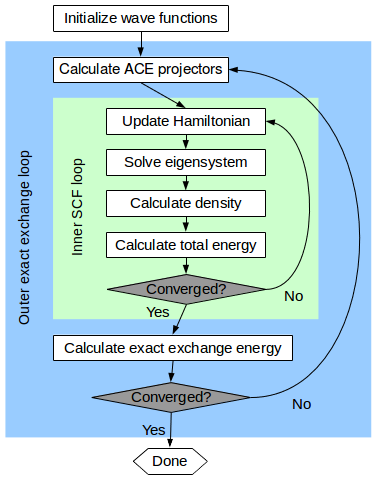
Fig. 221 A flowchart diagram showing the double self-consistency loop structure used in ACE hybrid functional calculations.
In QuantumATK ACE hybrid functional calculations therefore employs a double self-consistent loop
algorithm, see Fig. 221. Starting from a reasonable initial guess for the wave
functions \(|\psi_i\rangle\), we construct the ACE projectors and perform a regular DFT SCF
loop in which the ACE operators are added to the Hamiltonian and are kept constant. The resulting
wave functions are then used to update the ACE projectors and a new SCF loop is started. In this
way the ACE operator adaptively improves every outer iteration and the process is continued until
the exact exchange energy of the system is converged, in which case the ACE operator will be
identical to the real exact exchange operator [6]. The tolerance on the
exchange energy and the number of outer scf loops taken can be set on
IterationControlParameters.
Usage Examples
Running a calculation with HSE is as simple as setting the correct exchange_correlation
on the PlaneWaveCalculator. By choosing:
exchange_correlation = HybridGGA.HSE06
calculator = PlaneWaveCalculator(exchange_correlation=exchange_correlation)
the standard HSE06 parameters are chosen, i.e. screening_length=0.11*Bohr**-1
and exx_fraction=0.25.
One can set custom values for these parameters by choosing:
exchange_correlation = HybridGGA.HSECustom(screening_length=0.14*Bohr**-1, exx_fraction=0.20)
calculator = PlaneWaveCalculator(exchange_correlation=exchange_correlation)
By default the first SCF loop will have ACE projectors that are set to zero. In a lot of cases it makes sense to start from a PBE calculation, this can be done as follows:
calculator = PlaneWaveCalculator(exchange_correlation=GGA.PBE)
configuration.setCalculator(calculator)
configuration.update()

new_calculator = calculator()(exchange_correlation=HybridGGA.HSE06)
configuration.setCalculator(new_calculator, initial_state=configuration)
configuration.update()
When restarting, the wave functions of the old configuration will be used to construct ACE projectors, and an exact exchange contribution will already be present in the first SCF loop.