It is well known that DFT methods, or to be more specific the LDA and GGA exchange-correlation functionals, are not very adept at predicing the band gap of semiconductors.
They do, however, in many cases give rather accurate curvatures of the bands. We can use this to compute the effective mass of holes and electrons by fitting a parabola to the minimum/maximum of the conduction/valence bands.
The effective mass is a parameter that depends on several assumptions and definitions, so it will be important to properly understand the underlying concept, instead of just using it as a black box. For other materials, these assumptions may be different!
The lowest conduction band of Si has 6 equivalent minima, located along (101) (called \(\Delta\)) and its permuted equivalent directions in reciprocal space.
The minimum is located at (x,0,x) where x is about 0.425, or 85% of the distance to the first Brillouin zone boundary at X=(1/2,0,1/2).
At this point, the energy isosurfaces are ellipsoids, thus you get different values for the effective mass depending on if you look in the longitudinal (along ) or transverse (perpendicular to \(\Delta\)) directions. See Refs. [1] and [2] for more details.
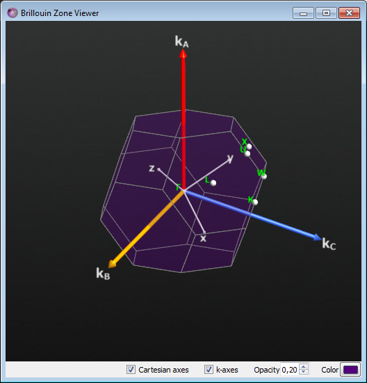
By (1/2,0,1/2) we mean a k-vector \(K=(\mathbf{G}_A+\mathbf{G}_C)/2\), where \(\mathbf{G}_A\), \(\mathbf{G}_B\), \(\mathbf{G}_C\) are the three unit vectors that span the reciprocal unit cell. If we express this point in Cartesian coordinates (still in reciprocal space) we find that the \(\Delta\) direction is parallel to \(\mathbf{K}_Y\). Obviously then, \(\mathbf{K}_X\) and \(\mathbf{K}_Z\), which are parallel to \(\mathbf{G}_B+\mathbf{G}_C\) and \(\mathbf{G}_A+\mathbf{G}_B\), respectively, are perpendicular to \(\mathbf{K}_Y\). Thus the transverse directions are (011) and (110), and the longitudinal one is (101) - see the figure below illustrating the Brillouin zone of silicon.
Fig. 29 Brillouin zone of silicon. In the Builder use Bulk Tools ‣ Brillouin Zone Viewer to visualize the Brillouin zone, fractional- and Cartesian directions and the high-symmetry points.
What we now need to do is:
generate a sequence of points \(k\) around a specified point \(k_0\), in a given direction;
compute the energy eigenvalues \(E(k)\) for the lowest conduction band for these \(k\)-points;
perform a numerical (finite difference) second order derivative of the band, \(d = \partial^2 E(k)/\partial k|_{k=k_0}\);
compute the effective mass as \(m^* = \hbar^2/(2d)\,m_e\) where \(m_e\) is the free electron mass.
If we do this for the longtitudinal (L) and transverse (T) directions, we will obtain three values, \(m^*_L\), \(m^*_{T1}\), and \(m^*_{T2}\) (actually, for Si \(m^*_{T1} = m^*_{T2} = m^*_{T}\)), which we can insert in the well-known expressions for the conductivity and density of states effective masses:
The first step is to do a self-consistent DFT calculation for Si.
The details involved in such a task are described in the Calculate the band structure of a crystal.
There, the extended Hückel method was used, so you should modify the calculator to use ATK-DFT instead.
Note that by default the LDA exchange correlation functional is used and you just need to specify a proper k-point mesh, i.e. 15x15x15.
Before saving and running your DFT calculation, you can set up the effective mass analysis directly from the Scripter.
Add Analysis ‣ EffectiveMass analysis after the calculator:
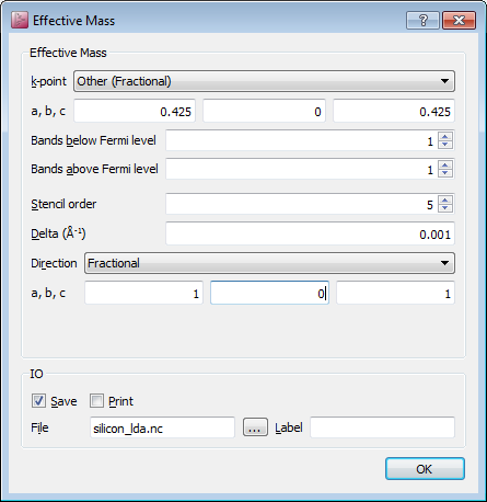
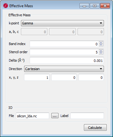
Double-click on EffectiveMass to set up the effective mass calculation. Here, you have several options and you can find all the details for each of these options in the EffectiveMass.
In order to calculate the effective mass at the conduction mass minimum enter the following parameters:
Change the k-point to “Other (Fractional)” and use the [0.425, 0, 0.425] coordinates.
Select one band above the Fermi level (conduction band only) and one band below the Fermi level. However, feel free to select as many bands as you wish!
As you will see later they will be conveniently listed in the LabFloor. Only remember that the effective masses calculated for all these bands correspond to the specified [0.425, 0, 0.425] point.
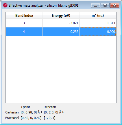
Set the Direction to Fractional and set a=1, b=0, c=1, corresponding to the longitudinal direction, c.f. Background.
Leave all the other default parameters.
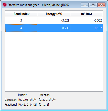
Add a second EffectiveMass analysis object with the same settings, except the direction which should be a=1, b=1, c=0, corresponding to one of the transverse directions.
Finally, set the output filename, silicon_lda.hdf5 for example, save and run the script.
The job will take just a few seconds.
You will now find the Bandstructure and EffectiveMass objects in the LabFloor. Let’s first check the bandstructure: double-click on it and use the Bandstructure Analyzer tool to plot it.
Inspecting the bandstructure it’s clear that the band gap is severly underestimated, but the shape is essentially correct; the gap is indirect and we do have a conduction band minimum at about 85% of the distance to X.
With these values we can now compute the density of states mass \(m^*_{DOS}=1.05\) and \(m^*_C=0.26\), very close indeed to the reference values 1.08 and 0.26 (see e.g. http://ecee.colorado.edu/~bart/book/effmass.htm ). Thus DFT actually does reproduce the effective mass of the electrons in the \(\Delta\) valley very well.
You may have noticed at the bottom right corner of the Bandstructure analyzer window the Effective mass button.
You do have indeed a second interactive tool at your disposal to calculate the effective masses.
This is a very convenient tool since you can select the k-point for which the effective mass will be calculated directly from the plot:
zoom in in the desired region of the plot and left-click to the desired point
Click on “Effective mass…” to open the effective mass tool:
Here, all the relevant parameters such as bandindex and k-point coordinates corresponding to the clicked point will be automatically set.
Note that you can change and refine these parameters.
Press “Calculate” to calculate the effective mass.
Check on the LabFloor where the Effective Mass object is stored and follow the steps above to get the effective mass.
The effective mass tools contain a couple of additional parameters which we have not mentioned.
Stencil order: it is possible to select the number of k-points that will be used to generate the band structure for which we perform the numerical derivative.
Delta: this parameter controls how far away from the chosen k-point we go. The default is typically fine; if the band structure is strongly non-parabolic, the value can be decreased a bit perhaps.
You can now also try the same calculation with the extended Hückel method.
If you followed the Calculate the band structure of a crystal you already have the necessary HDF5 file. The band minimum is not at x=0.452 this time, but closer to x=0.445. The results are very similar, however (\(m^*_L=1.00\) and \(m^*_T=0.17\)).
For Si, we compute a light hole mass (at the Γ point [0,0,0]) \(m^*_{LH}=-0.16\) (band index=1), and for the two degenerate heavy hole bands the result is \(m^*_{HH}=-0.25\) (band indices 2 and 3, respectively). These values are obtained in the directions of the Cartesian axes (i.e. if we use the same directions as for the electron, along \(\Delta\) from \(\Gamma\) to X). If, however, we look in the \(\Lambda\) direction from \(\Gamma\) to L (by setting the direction in the Analyzer to [1,1,1]), we find \(m^*_{HH}=-0.64\) and \(m^*_{LH}=-0.09\), a result of fact that the constant-energy surfaces for holes are strongly warped in Si, especially for the heavy hole bands [1][2].
To get proper hole masses that can be compared to experiments one should however also include spin-orbit interaction.