Molecular Device
Version: 2016.3
This tutorial focuses on the calculation and analysis of a molecular device. The device consists of a dithiol benzene (DTB) molecule (sometimes also called benzene dithiol, BDT) in contact with two gold (111) surfaces. This is a classic molecular device, sometimes called the fruit fly of molecular electronics, and it has been studied in a large number of publications, see for instance [1][2] and references therein.
Some of the calculations in this tutorial are quite time-consuming; for a quicker introduction to quantum transport studies with ATK, see Transport calculations with QuantumATK. The example structure you will use is a molecular junction with a benzene ring between two gold electrodes. You can find the instruction of how to build it in Molecular Junction.
The DFT model in QuantumATK is the underlying calculation engine used in this tutorial. A complete description of all the parameters, and in many cases a longer discussion about their physical relevance, can be found in the ATK reference manual.

Zero-bias calculation
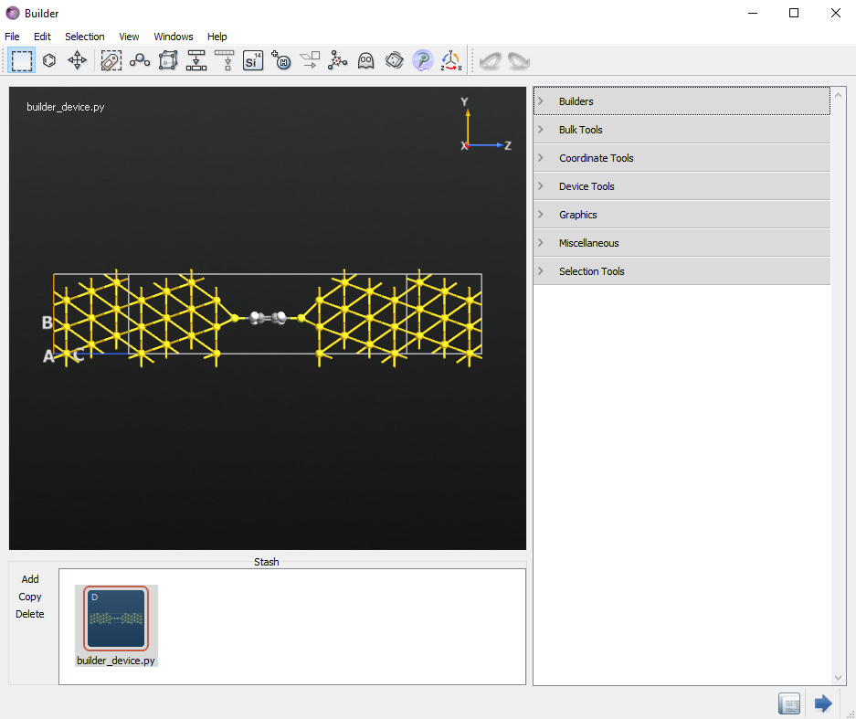
Following the instruction of Molecular Junction,
or download the script builder_device.py, you will get the following structure.
Attention
The geometry was not relaxed. This is not critical for the concepts we will discuss in this tutorial, but it is an important step to consider for any real calculations with ATK. To learn how to relax a device geometry, see the Relaxation of devices using the OptimizeDeviceConfiguration study object.
Setting up the calculation with the Script Generator
Now send the geometry to the Script Generator  by
pressing the Send to button
by
pressing the Send to button  at the lower right-hand corner of
the Builder and select Script Generator from the pop-up menu.
at the lower right-hand corner of
the Builder and select Script Generator from the pop-up menu.
In the Script Generator, add three blocks:
a New Calculator

an

an
Change the default output filename to
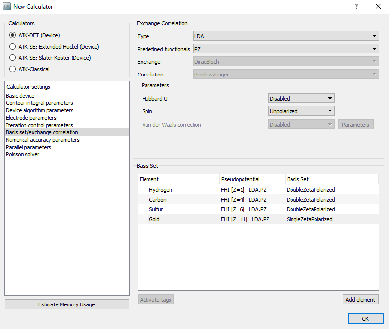
au-dtb-au.hdf5.Open the New Calculator
block and change the following
settings:Set the k-point sampling to 3 x 3 x 50 points.
In , reduce the basis set to SingleZetaPolarized for Gold to gain some speed.
Open the
DeviceDensityOfStates block by double-clicking
it and change the following settings:set the k-point sampling to 3 x 3 points
set the energy range to (-3, 3) eV
set points from 101 to 401
Open the
TransmissionSpectrum block and make the same
modifications, i.e.set the k-point sampling to 3 x 3 points.
set the energy range to (-3, 3) eV.
set points from 101 to 401
Finally, save the calculation script to the file
au_dtb_au.pyin your working directory for future reference. You can also download the fileau-dtb-au.pyfor comparison.
To run the script on your local machine, send it to the Job Manager
 by pressing the Send to button at the
lower right-hand corner of the Script Generator and select Job Manager
from the pop-up menu. In the Job Manager, press Run Queue to launch the
job. On a modern, single-node computer the script should take around an hour to
execute.
by pressing the Send to button at the
lower right-hand corner of the Script Generator and select Job Manager
from the pop-up menu. In the Job Manager, press Run Queue to launch the
job. On a modern, single-node computer the script should take around an hour to
execute.
Note
The calculation speed can be increased greatly by using a parallel computer. For information about how to run jobs in parallel, see the Parallelization of QuantumATK calculations.
Analysis of the zero-bias results
In this chapter you will extract data from the zero-bias calculation. You will do the following analyses:
Compare the transmission spectrum with the Partial Device Density Of States (PDDOS) of the phenylene ring.
Calculate the Molecular Projected Self-Consistent Hamiltonian (MPSH), and rationalize the transmission in terms of the MPSH states.
Calculate the transmission eigenstates.
Calculate the energy-dependent Local Density of States (LDOS), in order to obtain a spatial view of the energy levels.
The transmission spectrum and density of states
Return to the main QuantumATK window. The au-dtb-au.hdf5 file should now be
visible under Project Files, and its contents displayed on the LabFloor.
It contains three objects:
 DeviceConfiguration contains the two-probe device
configuration and the self-consistent state of the attached calculator.
DeviceConfiguration contains the two-probe device
configuration and the self-consistent state of the attached calculator. TransmissionSpectrum contains all information
about the computed transmission spectrum, including settings and results.
TransmissionSpectrum contains all information
about the computed transmission spectrum, including settings and results. DeviceDensityOfState contains all
informations about the Density state of the device region.
DeviceDensityOfState contains all
informations about the Density state of the device region.
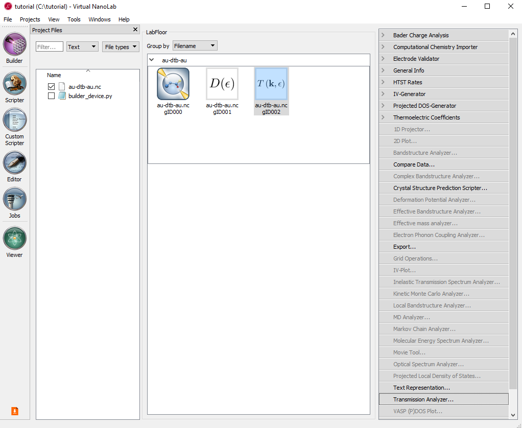
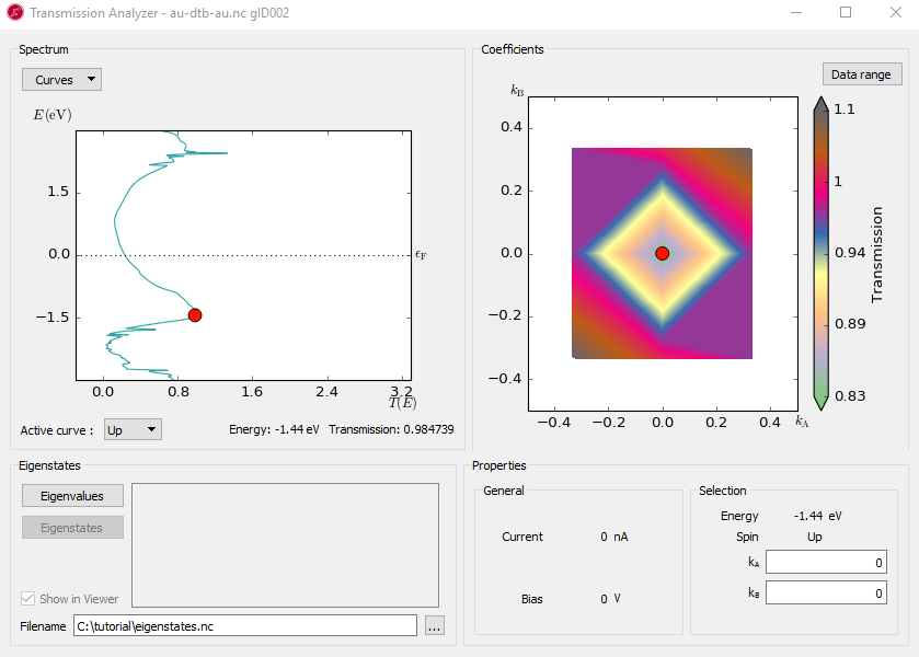
Select the TransmissionSpectrum object, and click the Transmission Analyzer in the right-hand panel bar.
The Transmission Analyzer plugin opens. On the left, named Spectrum, is shown the k-point averaged transmission spectrum as function of energy. The average Fermi energy of the two electrodes is set to zero and indicated with a dashed line.
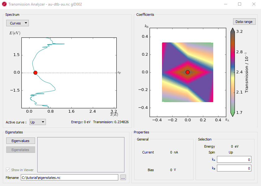
Fig. 104 The k-point averaged transmission spectrum as function of energy
The transmission and energy values in the point marked by the red dot are shown below the plot. You can use the mouse to move the dot along the \(T(E)\) curve and read off the values. The Curves drop-down menu lets you select the spin components to be plotted. Note that the transmission for spin types X, Y, and Z are only non-zero for calculations with noncollinear spin.
At any particular energy (defined by the red dot), the total transmission is computed as an average over the transmission coefficients in the sampled k-points. The right-hand plot, named Coefficients, shows an interpolated contour plot of the transmission coefficients vs. reciprocal vectors \(k_A\) and \(k_B\). For example, at the energy, E = -1.4 eV, where you find a spectrum peak at the transmission, the contribution is minimum around the \(\Gamma\) point, as shown in the figure below.
There are three broad peaks, at around -3, -1.4 and 2.5 eV. Also note the narrow peak around 2.4 eV which rises above T(E)=1. In the following you will investigate the origin of these peaks.
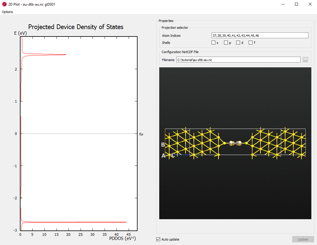
Next select the DeviceDensityOfStates object and
click the button to open the PDDOS analyzer
window.To merge both PDDOS lines into one, click the Options button on the
upper left corner and turning off flipping.
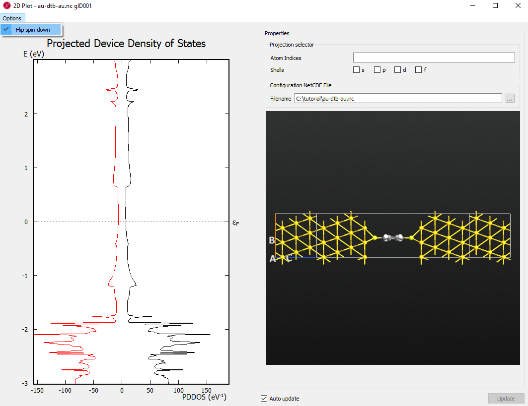
Select all carbon and hydrogen atoms by enclosing them with a rectangle using left mouse button (or select the individual atoms with Ctrl left-click).
Tip
Copy the Atom Indices here as you will need to input the indices in the next step.
Note
The similarity in the peak structure of the PDDOS and the transmission spectrum indicates a clear correspondence between the energy levels on the phenylene ring and the transmission spectrum.
The Molecular Projected Self-Consistent Hamiltonian (MPSH)
To understand the energy levels of the phenylene ring in the presence of the surrounding electrodes, you will now calculated the MPSH states. The MPSH states are obtained by diagonalizing the molecular part of the full self-consistent Hamiltonian [1].
Open the Script Generator tool and
Double-click Analysis from File to add the block
 .
.Select the file
au-dtb-au.hdf5, then select .Add .
Change the output filename to
dtb_analysis.hdf5.Open the MolecularEnergySpectrum block
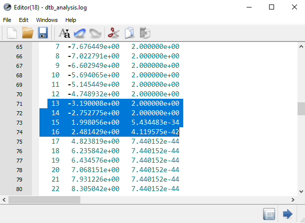
and input the
indices of carbon and hydrogen atoms to Atom indices (37,38,39,40,41,42,43,44,45,46).
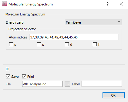
Send the script to the Job Manager
and execute it (the
execution only takes a few seconds). The MPSH energies are then printed in
the log file.
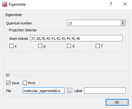
To calculate the eigenstates of the MPSH levels, reopen the last Script Generator
(it is available from the windows menu at the top of each
QuantumATK window, if you didn’t close it).
Change the name of the output file to
molecular_eigenstate.hdf5.Add four
blocks.Open each EigenState script block and select projection on carbon and hydrogen Set the Quantum number to 13, 14, 15, 16 in each respective block.
You may delete the MolecularEnergySpectrum block
, it is no
longer needed (select it and press the Delete key).Send the script to the Job Manager
and execute the script.
When the calculation is done, the molecular_eigenstate.hdf5 file should
already be ticked under the Project Files, so its objects will appear on the
LabFloor. Select the first eigenstate object. Click the button
in the tool bar on the right-hand side and select
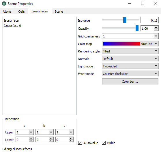
Isosurface. In the Viewer, open the Properties menu, select the
tab and do the following settings.
Set the Isovalue to 0.16.
Set the Color map to BlueRed
Tick \(\pm\) Isovalue
To visualize the eigenstate together with geometry, drag and drop the file
builder_device.py onto the Viewer. Do the same to the other eigenstates
and you will get the figures below:
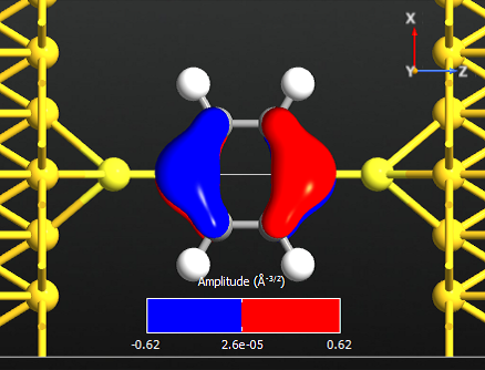
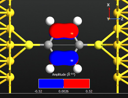
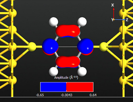
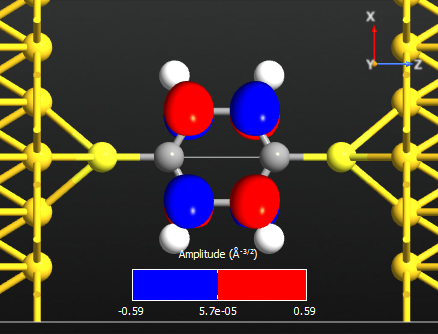
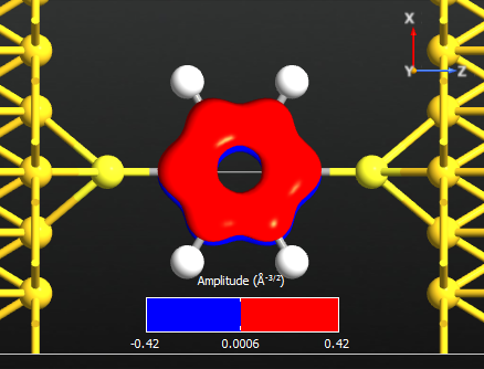
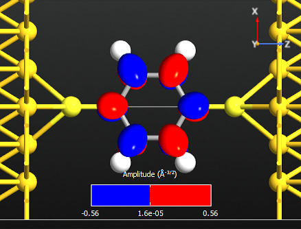
Note that all the states are anti-symmetric in the plane of the benzene ring. This means that they are the \(\pi\)-orbitals of the benzene ring, i.e. they are linear combinations of the p-orbitals on each carbon atom which are perpendicular to the plane of the molecule. There are 6 such p-orbitals which means that there are 6 \(\pi\)-orbitals.
By visually inspecting the symmetry of the different eigenstates the remaining
two \(\pi\)-orbitals are identified as state 10 and 18. Use Editor
 to open the previous script, delete two Eigenstate blocks and change
the quantum_number in the remaining two Eigenstate blocks to be 10 and 18
respectively. These are visualized below with an iso-value of 0.16.
to open the previous script, delete two Eigenstate blocks and change
the quantum_number in the remaining two Eigenstate blocks to be 10 and 18
respectively. These are visualized below with an iso-value of 0.16.
Note
There are 6 electrons in the \(\pi\)-band, corresponding to that lowest 3 states are occupied. We may therefore denote state 14 the HOMO and state 15 the LUMO.
Transmission eigenvalues and eigenstates
In this chapter you will analyze the transmission eigenstates at the peak positions in the transmission spectrum, i.e. at energies -3, -1.5 and 2.4 eV.
Re-open the Script Generator
and delete the
Eigenstate blocks .Instead, add three
blocks.Set the energies to -3, -1.5 and 2.4 eV, into the three TransmissionEigenvalues blocks
respectively.Execute the script using the Job Manager
and inspect the log file.
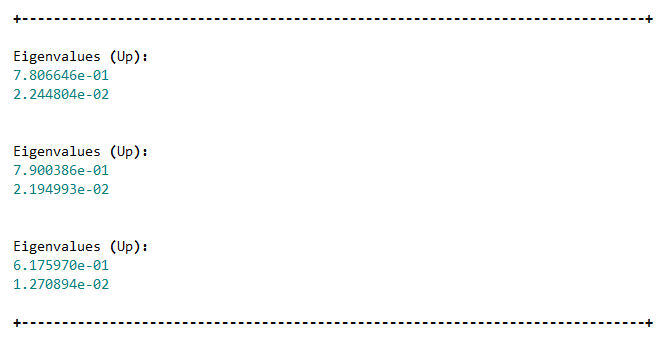
The transmission eigenvalues are obtained by diagonalizing the transmission matrix. The number of eigenvalues indicates the number of individual channels through the molecule, and the eigenvalue shows the strength of each channel. The eigenvalues are the true transmission probabilities, and thus lie in the interval [0,1]. If several channels are available at a particular energy, their sum - and hence the transmission coefficient at this energy - may however be larger than 1.
Most of the eigenvalues are very small and can be neglected. The two largest eigenvalues of each energy are the most important ones.
Note
At the first two energies there is only one dominating eigenstate, while at the last energy there are two dominating eigenvalues. The reason that they do not sum up to the total transmission spectrum T(E) will be discussed in the next section.
The next step is to visualize the transmission eigenstates for the first two peak energies, where there is only one significant eigenvalue.
Re-open the Script Generator
and delete the
TransmissionEigenvalues blocks .Add two
blocks.Enter the energies -3 and -1.5 into the blocks
. Leave the quantum number at
0, corresponding to the highest eigenvalue.Execute the script via the Job Manager
.
The objects will again be saved in the file dtb_analysis.hdf5 and can be
visualized using the same approach as for the eigenstates. Below are shown
isosurfaces of the two transmission eigenstates.
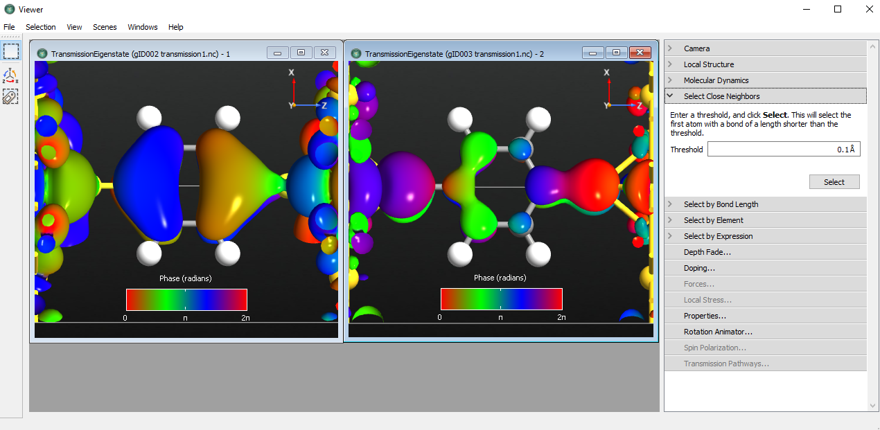
Fig. 105 Transmission eigenstates of energy -3 and -1.5 eV
Tip
The transmission eigenstate is a complex wave function. The isosurface shows the absolute value of the wave function while the color of the isosurface indicates the phase. Since the phase is periodic, it is best to use a periodic color map.
The transmission eigenstate at -3.0 eV has a clear resemblance with MPSH state 13, i.e. the HOMO-1 state. The transmission eigenstate at -1.5 eV is also a \(\pi\)-state.
k-dependent transmission and eigenchannels
You will now analyze the transmission at 2.4 eV. Previously, you found that there is an important transmission eigenstate at this energy with transmission probability 0.618 which is different from the value 1.45 obtained from inspecting Fig. 104. This is because Fig. 104 shows the k-point averaged transmission. You will now calculate the k-dependent transmission coefficients at this energy.
Re-open the Script Generator
and delete the
TransmissionEigenstates blocks.Add an block
.Open the TransmissionSpectrum block
and setEnergy start and end equally to 2.4 eV,
Number of energy points to 1,
k-point sampling to 21 x 21 points,
Execute the script using the Job Manager
.
When the calculation has finished you can visualize the k-dependent using .
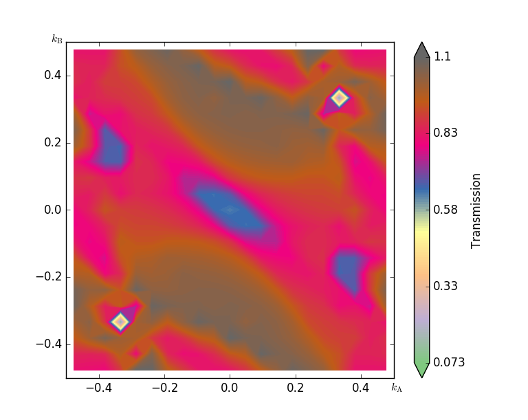
Fig. 106 The k-dependence of transmission at energy point 2.4eV
The contour plot of the k-dependent transmission above has a pronounced peak at \((k_A,k_B)=(0.0,0.38)\), with a transmission coefficient of around 1. In the computation of the transmission spectrum earlier, we did not have a dense enough k-point sampling, and hence the transmission was overestimated, i.e. we obtained 1.45 while the 21x21 mesh gives around 1.1.
Attention
This shows the importance of carefully checking the convergence of the results in the k-point sampling of the transmission spectrum. There is no reason to assume that the same number of points used to get a correct electron density (i.e. the k-points used in the self-consistent calculation) also give an accurate transmission.
You will now calculate the transmission eigenstates at the k-point with the strongest transmission. We can choose either point (0, -0.38) or (0, 0.38), they are equivalent by time-reversal symmetry.
Click the point (0, -0.38) or (0, 0.38) on the transmission contour plot.
Click in the Eigenstates block on the lower left side. You will get a list of eigenvalues.
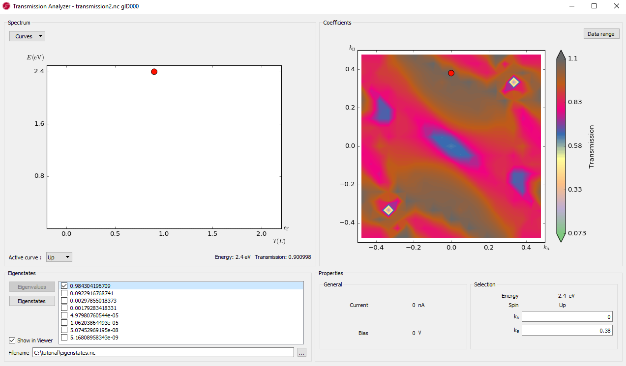
Select the first eigenvalue only, and press the button . The first eigenstate will be calculated and the Viewer window will pop up with a figure. Tune the isovalue in to display the eigenvalue image nicely.
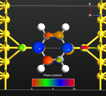
Fig. 107 The first eigenstate contributes to the transmission at energy point 2.4 eV.
Projected local DOS
In this section you will calculate the local device density of states throughout the device, projected onto the real-space transport direction (the Z-axis).
Re-open the
Script Generator and delete the
previous analysis blocks.Add a
block.Open the analysis block and edit it: Increase the energy window to -3 eV to +3 eV, and set the k-point sampling to 3x3.
Change the output filename to
pldos_0.0V.hdf5and save the QuantumATK Python script aspldos_0.0V.py.
Execute the script – the calculations may take up to an hour to run. The PLDOS item will be added to the QuantumATK LabFloor. Plot the results using the Projected Local Density of States plugin in the right-hand plugins menu. Adjust the data range to get a plot like the one shown below.
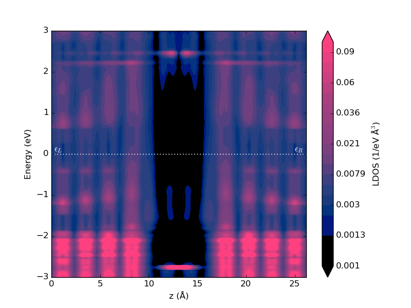
Fig. 108 Local device density of states projected onto the device Z-axis.
The PLDOS shows a high density in the metallic gold electrodes (pink regions), while the black color in the middle corresponds to vanishing DOS in the vacuum gap between the electrodes. In the middle, where the molecule is, there are three peaks in the local DOS as a function of energy, positioned around -3, -1.4, and +2.5 eV, in agreement with the peaks in the transmission spectrum.
I-V characteristics
In this chapter you will calculate the I-V characteristics of the Au-DTB-Au molecular device, and analyze the device for an applied bias of 1.6 V.
Setting up the calculation
Open a new Script Generator window, and do the
following:
Add the Analysis from File
block.Add the
block.Change the default output filename to
IV-curve.hdf5.
Edit the Analysis from File block:
Set HDF5 file to
au-dtb-au.hdf5, and use gID000 to restart from the zero-bias calculation.
Also edit the IVCurve block:
Set the voltage bias range to end at V0 = -2V and V1 = 2 eV.
Set the number of voltage points to 11.
Set the energy range as (-3,3).
Use 3x3 transverse k-points.
Choose the Krylov self-energy calculator (for speed).
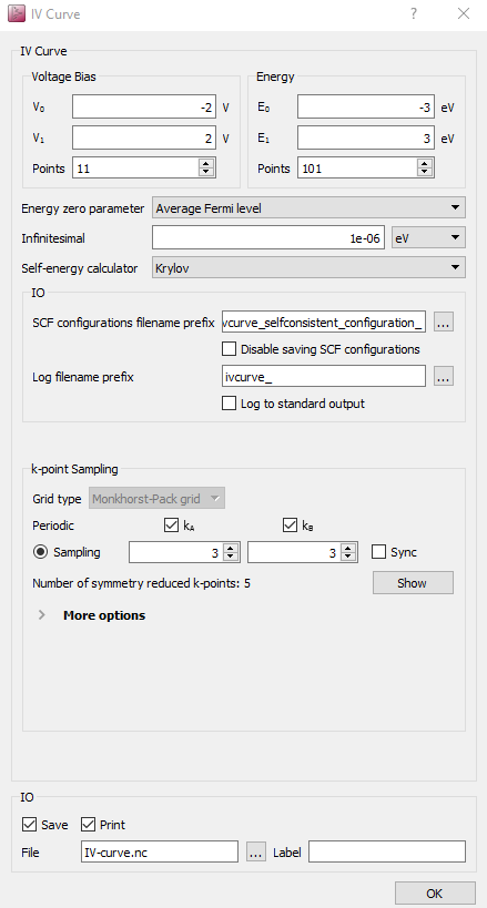
The script is now done. Save it as iv-curve.py and execute it using
the Job Manager or from the command line. This
calculation will take some time, because a self-consistent SCF calculation
and a transmission spectrum analysis must be done at each bias point. It takes
six hours to finish in a 12-core machine.
IV characteristic analyzation
Once the calculation is done, the file IV-curve.hdf5 appears in the folder.
Eleven new output files are also created, prefixed ivcurve; they contain
the converged SCF state at each bias point.
Note
 The IVCurve object contains the calculated I–V curve,
including the transmission spectra computed at each bias voltage.
The IVCurve object contains the calculated I–V curve,
including the transmission spectra computed at each bias voltage.
Select the IV-curve and click the IV-Plot analysis tool in the right-hand plugins bar. The I–V curve is plotted in the window that pops up.
Check the box Additional plots. Three additional panels appear, plotting the differential conductance (dI/dV), the calculated transmission spectra, and the spectral current.
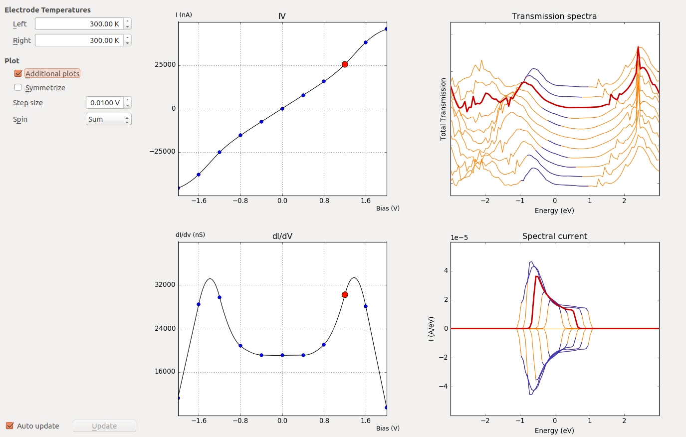
Fig. 109 Each transmission spectrum and spectral current correspond to a specific bias voltage point. The energy range corresponding to the bias window is indicated in blue. By moving the mouse cursor to one of the marker points on either the IV or dI/dV plot, the corresponding transmission spectrum and spectral current will be highlighted.
Attention
Pay special attention to the spectral current: All possible contributions to the total current must be included inside the specified energy window, in order to get accurate \(I(V)\) points. If this is not the case, you should consider redoing the analysis using a wider energy window.
Note
The peak in the dI/dV around 1.6 V arises from a resonance in the transmission spectrum entering the bias window at this voltage.
PLDOS at 1.6 V bias
To investigate in details the electronic features of the molecular device under bias of 1.6V, you should compute the projected local density of states, just like you did above for zero bias, in section Projected local DOS.
Open a new script by cliking Script Generator
and
add two blocks:Select file
ivcurve_selfconsistent_configuration_1.60000V.hdf5from the previous calculation after opening the block.In the PLDOS analysis block, increase the energy window to -3 eV to +3 eV, and set the k-point sampling to 3x3.
Change the output filename to
pldos_1.6V.hdf5and save the QuantumATK Python script aspldos_1.6V.py.
Run the script and use agin the Projected Local Density of States plugin to visualize the results.
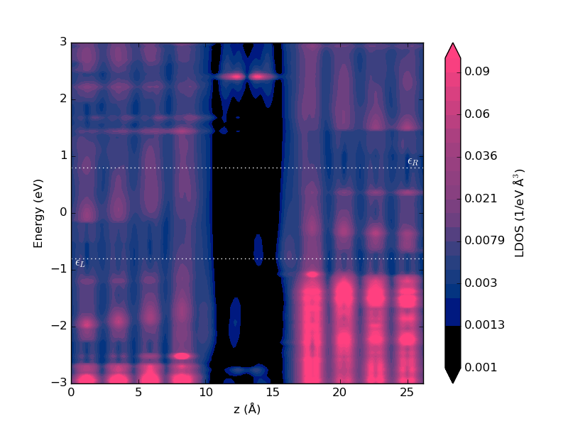
Fig. 110 Projected local device DOS at 1.6 V applied bias.
Compared with Fig. 110, the resonance at -1.5 eV has split into two resonances, at -0.8 and -2 eV, as we saw already in the transmission spectrum above. We also see that the resonance at -0.8 is located towards the right electrode, while the resonance at -2 eV is located towards the left electrode. The splitting arises from the drop in the electrostatic potential through the molecule (due to the applied bias), as will be investigated in the next section.
Calculating the voltage drop
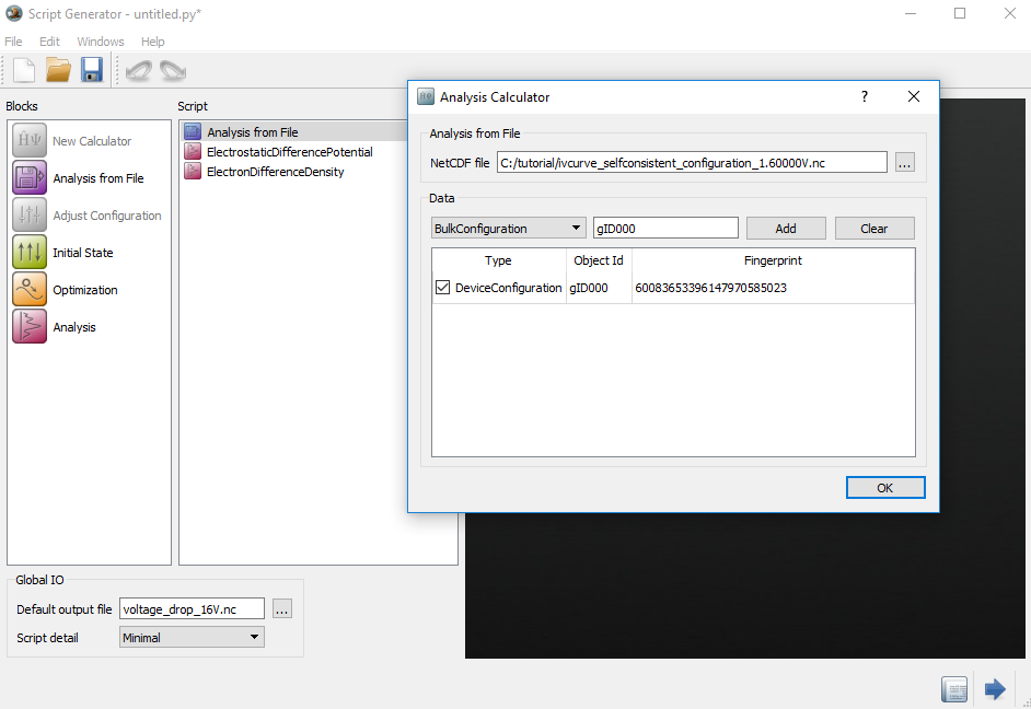
You will now calculate the voltage drop and induced density for an applied bias of 1.6 V. At first, we will calculate the ElectrostaticDifferencePotential and ElectronDifferenceDensity between 1.6 V and 0 V.
In the Script Generator
, add three blocks:the Analysis from File
an
an
Open the Analysis from File
to load the ivcurve_selfconsistent_configuration_1.60000V.hdf5.Change the default output filename to
voltage_drop_16V.hdf5.Send it to the Job Manager
by pressing the Send to button.
Repeat the above recipe to calculate the ElectrostaticDifferencePotential
and ElectronDifferenceDensity at 0 V. Finally, you will have the files
voltage_drop_16V.hdf5 and voltage_drop_0V.hdf5 under
Project files.
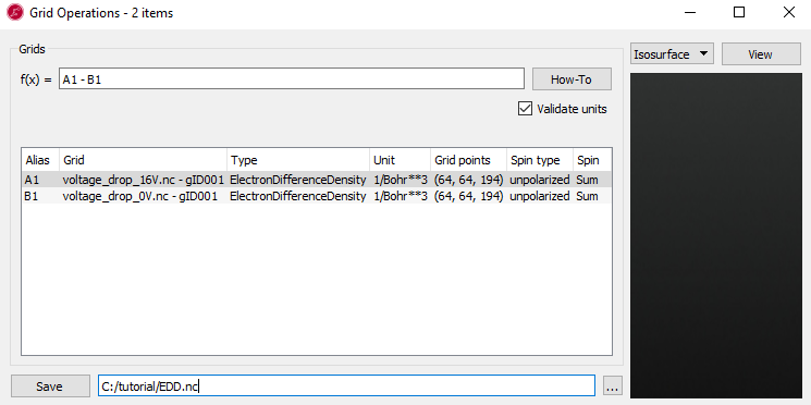
To calculate the voltage drop using the ElectrostaticDifferencePotential and ElectronDifferenceDensity at 1.6 V and 0 V, we use GridOperations in the right-hand panel bar.
Select the two objects by holding the
ctrlkey while clicking on each \(\delta V_E(\mathbf{r})\) icon in thevoltage_drop_16Vandvoltage_drop_0Vfiles on the LabFloor.Open the GridOperations widget.
Make a function such as A1 - B1.
Save as
EDP.hdf5.
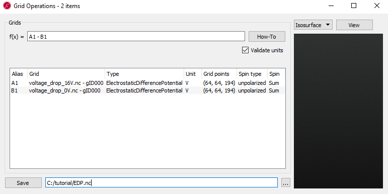
Repeat the above process for the density to get the voltage-induced density.
You should now have the calculated grids in the files EDP.hdf5 and
EDD.hdf5. To visualize the ElectrostaticDifferencePotential and
ElectronDifferenceDensity induced by the 1.6 voltage, do the following:
Select the file
EDP.hdf5and open the Viewer in the panel.Change the plot type in the grid visualization selection to the CutPlanes.
Drag the
builder_device.pyon the window.Next, select the file
EDD.hdf5and drag into the same window.Keep the default, Isosurface for the ElectronDifferenceDensity.
You can tune the CutPlanes and Isosurface in the properties. In the case of CutPlanes, you can adjust the 3D and position of the CutPlane.
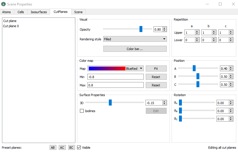
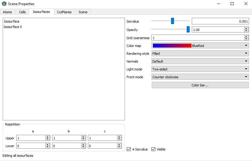
If you apply the settings shown above, you should now have the following figure:
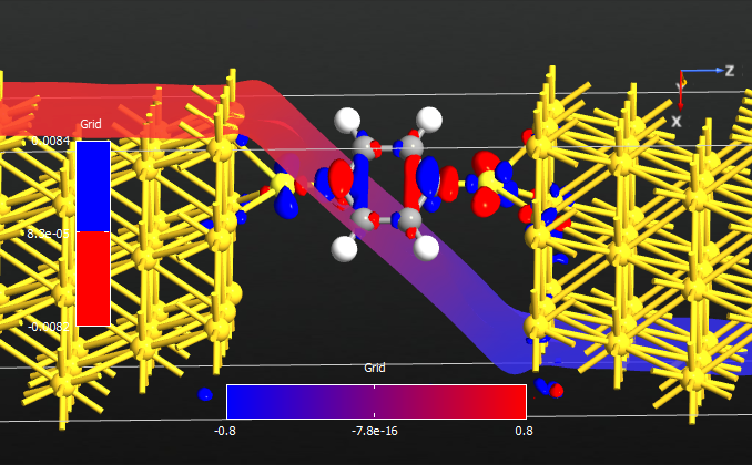
Fig. 111 Electrostatic potential drop and electron density difference induced by a bias of 1.6V.
It is useful to make a 1D plot of the voltage drop. To this end, select the \(f(x)\) of the EDP in the LabFloor and click the 1D Projector in the right hand panel bar. Then change the projection type to Average and click Add line.
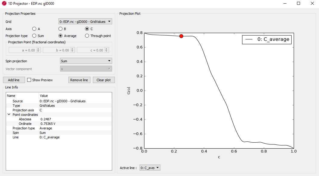
Fig. 112 Voltage drop along a line through the molecular axis.
In the case of 1D projection plot, c-axis shows the relative length between 0 and 1 corresponding to the real z distance.
Note
Both Fig. 111 and Fig. 112 show the total voltage drop of 1.6 V across the device. It is also clear from both figures that most of the voltage drop takes place around the molecule, not in the electrodes. A drop in voltage corresponds to a quantum resistance, and this explains the observed finite-bias splitting of the zero-bias resonance.