Interfacial thermal conductance
Version: 2016.1
The continuous downsizing of modern electronic devices implies the increasing complexity of a nano-device. The thermal conductivity is hard to predict when the device is formed by more than one material. More often, device engineers want to maximize or minimize the thermal conductivity by constructing interfaces between different materials.
In this tutorial, you will learn how to use molecular dynamics with a classical potential to simulate the heat flow through an interface and calculate the interfacial thermal resistance.

Introduction
You will simulate the heat current through a model grain boundary in a silicon crystal by imposing a temperature gradient between a heat source and a heat sink.
Theory
With a given temperature gradient, the bulk heat conductivity \(\kappa_{bulk}\) of a material is related to the heat flux via the Fourier equation,
where \(\langle dQ/dt \rangle\) represents the average heat flux (i.e. transferred kinetic energy per time) along the gradient, and \(A\) is the area perpendicular to the direction of the heat flux.
The presence of an interface between the temperature source and sink often causes a discontinuity (a temperature “jump”) \(\Delta T\) in the temperature profile, since the interface provides additional thermal resistance \(R\) to the heat current. In this case, the interfacial thermal conductance \(G\), often referred to as Kapitza conductance, can be defined as
Note
Sometimes it makes sense to normalize \(G\) to the cross-sectional area, e.g. if you want to compare similar interfaces with different cross sectional areas.
Method
In this tutorial, we will use two different methods to calculate the heat conductivity. In the first section, we will use molecular dynamics simulations, and in the second section we will use the non-equilibrium Green’s function method.
Reverse non-equilibrium molecular dynamics (RNEMD)
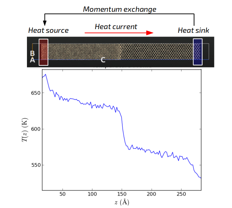
When using molecular dynamics (MD) simulations, the most common technique to impose a temperature gradient in MD simulations is the so-called non-equilibrium momentum exchange or reverse non-equilibrium molecular dynamics (RNEMD) method [1][2]. In this method two groups of atoms are selected as the heat source and the sink, respectively. During the simulation the momenta of the hottest atom in the sink and the coldest atom in the source are exchanged according to special criteria to conserve the total energy and momentum [2]. This external heat flux is balanced by a heat current from source to sink within the system, causing a measurable temperature gradient (and a temperature jump if an interface is present).
Preparing the grain boundary
You will consider a model grain boundary between two silicon crystal grains with different orientations. Although you can direct the thermal current in any arbitrary direction during the simulation, we will preserve the convention that current runs along the z-direction. Therefore, while building the system you should always make sure that the interface configuration is oriented correctly. If necessary, you should rotate the system to make sure the thermal current is oriented along the z-axis.
You will create an interface between a (100) and a (110) silicon surface.
Open the Builder  , and add Silicon (alpha) via
, and
, and add Silicon (alpha) via
, and
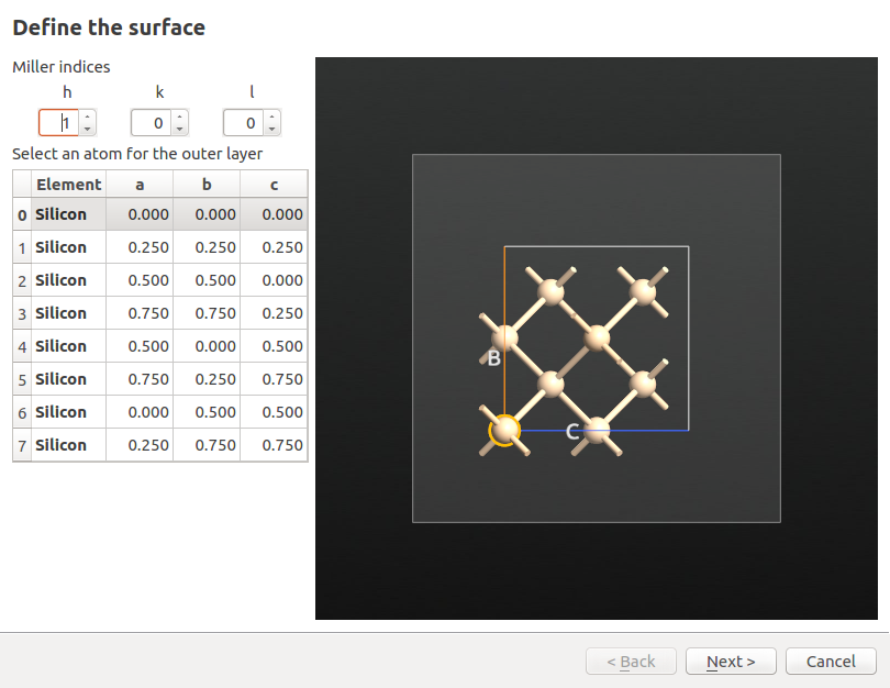
To generate a (100) surface base cell make sure the newly added Silicon alpha configuration is selected and,
Open the in the right-hand-panel under Builders.
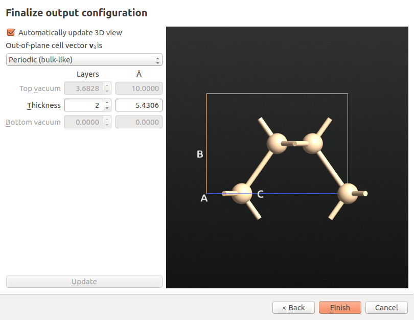
Select the (100) Miller indices, click Next, leave the 1x1 surface lattice, click Next, and select Periodic (bulk-like).
Click Finish to complete the surface creation.
Repeat the above steps for the (110) structure.
To avoid a large strain when joining the two cells with different lattice constants, you should choose suitable repetitions to obtain commensurate cell sizes. The cell sizes can be looked up and modified under .
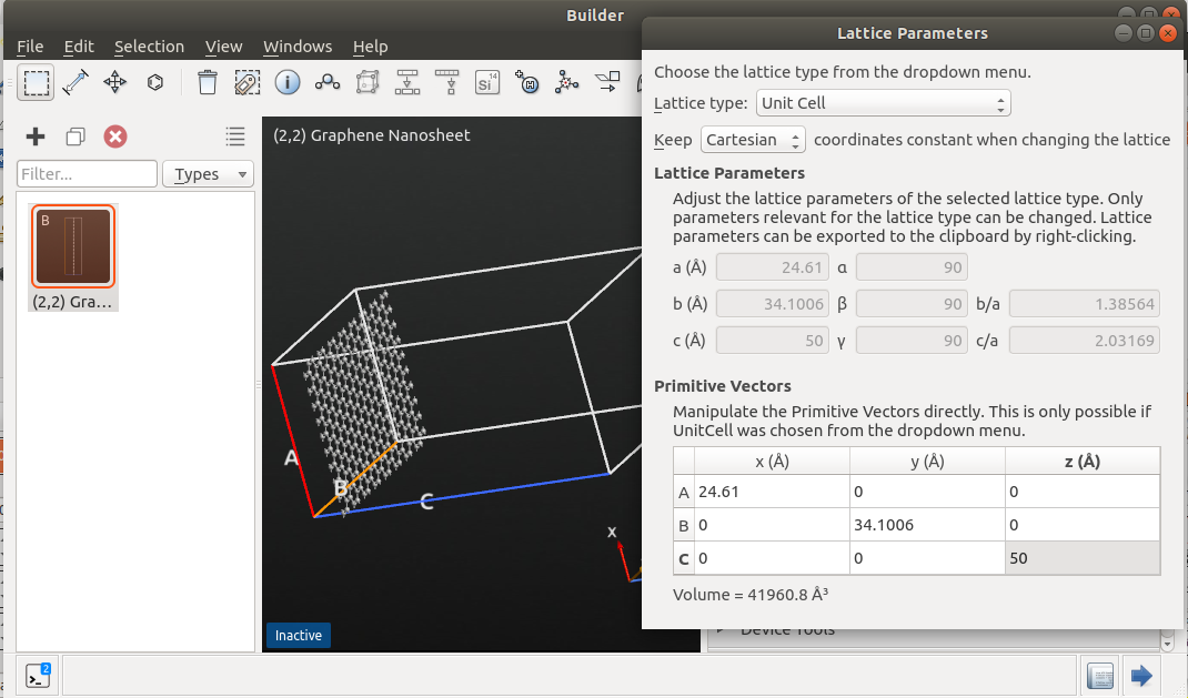
The cell of the (100) surface has dimensions 3.84 x 3.84 x 5.43 Å3, while the (110) cell has a size of 3.84 x 5.43 x 3.84 Å3. Therefore, a 3 x 3 x 12 repetition for the (100) cell, and a 3 x 2 x 17 repetition for the (110) cell, provides supercells of almost equivalent sizes. You can apply such repetitions using the . Set the desired number of repeats and click Apply.
Note
Generally, for such non-equilibrium thermal current simulations it is important to choose a sufficient cell length in the direction of the heat flow (in this case the C-vector), whereas the results are less sensitive to the geometry of the cross-sectional area (i.e. A x B). Therefore, the simulation cells employed typically have a stick-like shape.
Creating an interface with two structures could be a tedious task, but the Interface Builder helps you to complete it in a simple and flexible manner. Open in the right-hand-panel and drag and drop the (100) supercell onto the left field and the (110) supercell onto the right field.
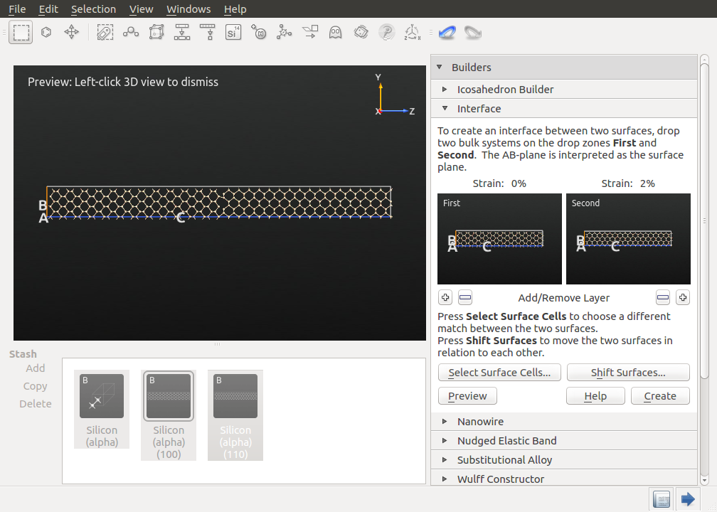
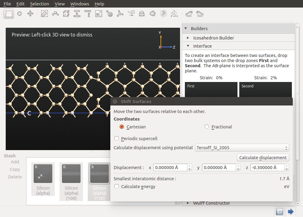
The preview of the interface should appear automatically (if not click Preview). If you zoom into the interface, you will notice a gap between the two surfaces. You can adjust this gap by clicking Shift Surfaces and adding a negative offset in the z-direction until bonds between the two surfaces are displayed. Moreover, you can align the two surfaces in the x and y-directions, as well. The proposed values should provide a good initial structure. Close the Shift Surfaces tool and click Create to create the interface structure.
Note
The displayed bonds are visual guides only and do not have a strict physical meaning. For the interface creation the appearance of bonds simply indicates if the initial guess is reasonable. The interface will be optimized, annealed, and equilibrated using molecular dynamics to reduce spurious features to the largest extent.
The supercell in this calculation should be non-periodic in the C-direction, meaning that the system is terminated by vacuum at either end. The lateral dimensions (A and B) will remain periodic.
To obtain such a setup, simply increase the length of the C-vector. This can be done by opening and increasing the \(C_z\) entry from about 130 Å to 160 Å. Make sure that you keep the Cartesian coordinates.
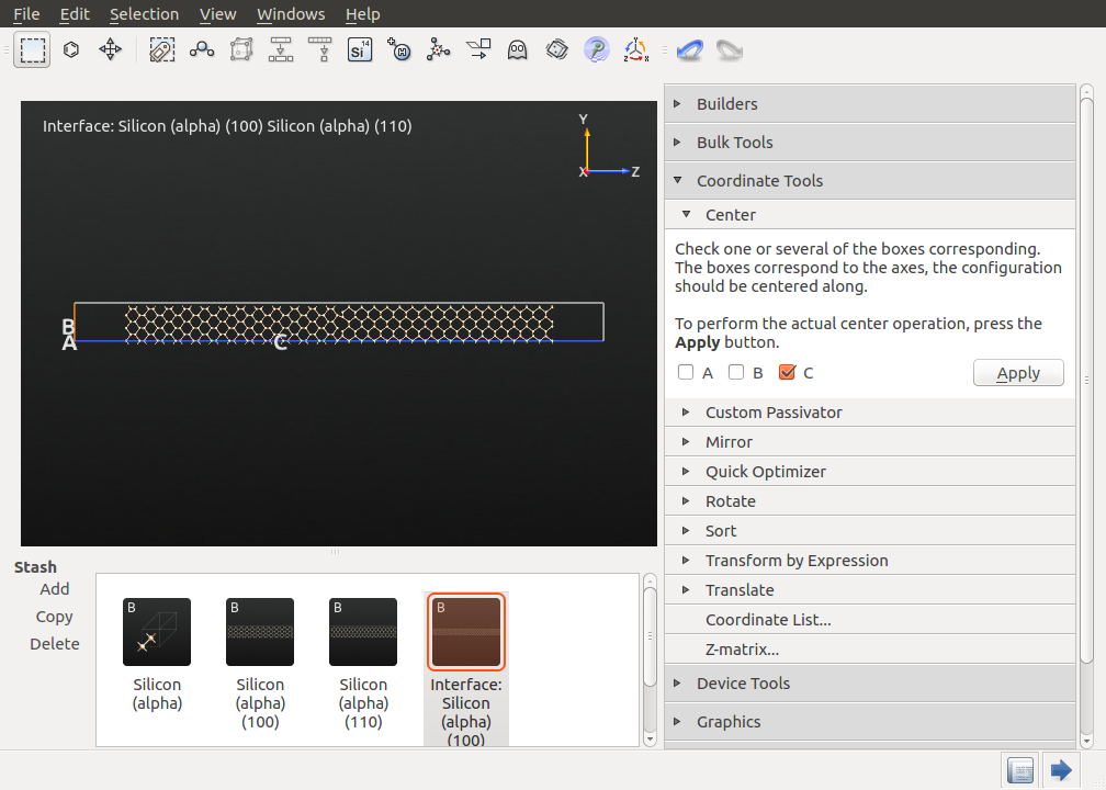
Finally, the slab should be centered in the middle of the supercell. Therefore, open , uncheck A and B and click Apply. The result should look like below.
Setting up the equilibration simulation
Prior to simulating the actual heat flow, the system has to be equilibrated
properly in order to reduce artifical defects due to the interface generation,
remove the lateral stress, and prepare a system which is equilibrated at the
desired target temperature. To do this, send the final interface to
the Script Generator  by clicking the Send To icon
 , and add 3 blocks:
 New Calculator
-
Change the Default output file name to Silicon_grain_boundary.nc,
and open the New Calculator block.
Select and the .
Uncheck and close the widget by clicking OK.
Note
For QuantumATK-versions older than 2017, the ATK-ForceField calculator can be found under the name ATK-Classical.
Open the OptimizeGeometry block and set the Force
tolerance to 0.1 eV / Å. The remaining parameters can
be left at their default values. Uncheck and
close the widget.
Note
The optimization is necessary to remove initial large destabilizing forces that might occur after the interface generation. As an interfaced is introduced, a small force is most likely unavoidable.
The next step is to allow the lateral cell vectors to relax and equilibrate
to the target temperature using the Molecular Dynamics method. The entire
thermal transport simulation will be performed at an average temperature
of 600 K. To do this, open the MolecularDynamics
block to set up the parameter for the NPT simulation, i.e. a simulation at
constant temperature and pressure.
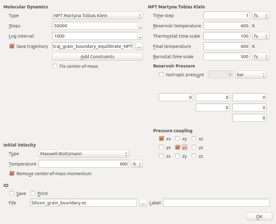
Select the Type as NPT Martyna-Tobias-Klein.
Set the number of steps to 50 000 and the log interval to 1000.
Choose a suitable trajectory name, e.g.
traj_grain_boundary_equilibrate_NPT.nc.Set the Reservoir temperature to 600 K, and the External stress to 0 bar.
Uncheck Isotropic pressure and disable the Stress coupling in the zz-direction, as the free surface in this direction will automatically adjust.
Select the Maxwell-Boltzmann-Distribution under Initial Velocity, set the temperature to 600 K, and make sure the box is checked to remove the center-of-mass momentum.
Uncheck , as the trajectory is saved anyway.
The final settings should look like the following.
Send the script to the JobManager  , save as
grain_boundary_equilibrate_NPT.py when asked, and run it.
We will use the resulting structure from the NPT simulation for the following
simulations. To this end, once the simulation has finished, select the trajectory on
the Lab floor in the main QuantumATK window
and open it with the Movie Tool. Play the trajectory and send the last snapshot
to the Builder using the icon.
Setting up the non-equilibrium momentum exchange simulation
You now have to define the regions for the heat source and sink in the heat current simulations. Zoom into the left end of the configuration and select the last 4 atom layers (i.e. the first unit cell), as shown in the picture below.
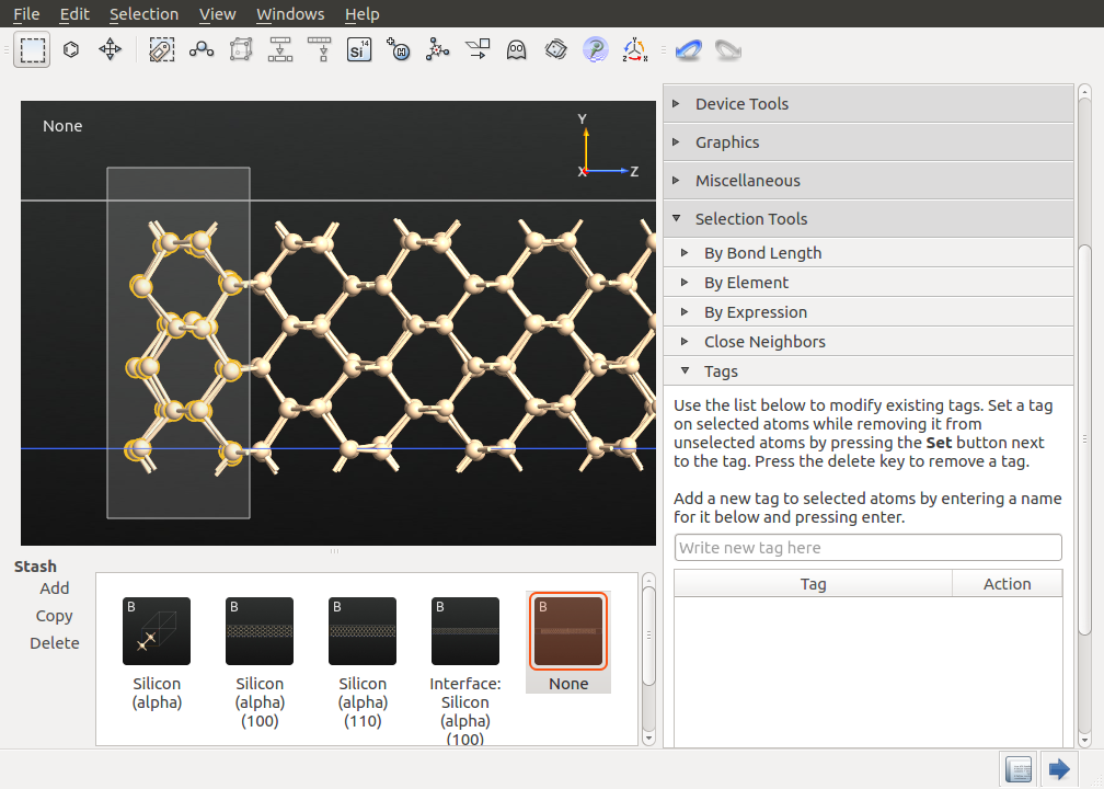
Open the plugin, enter a suitable tag name, e.g. heat_source, and press Return. The selected atoms will now be marked by this tag name and can be referred to during the simulation.
Repeat the same procedure at the other end of the configuration. Use a different tag name this time, e.g heat_sink.
Send the configuration to the Script Generator ,
add a New Calculator and two
MolecularDynamics blocks.
Edit the calculator block in the same way as described above, i.e. selecting with the .
First, you will perform another equilibration simulation at 600 K, this time
at constant volume, to prepare a well equilibrated system. Open the first
MolecularDynamics block, and,
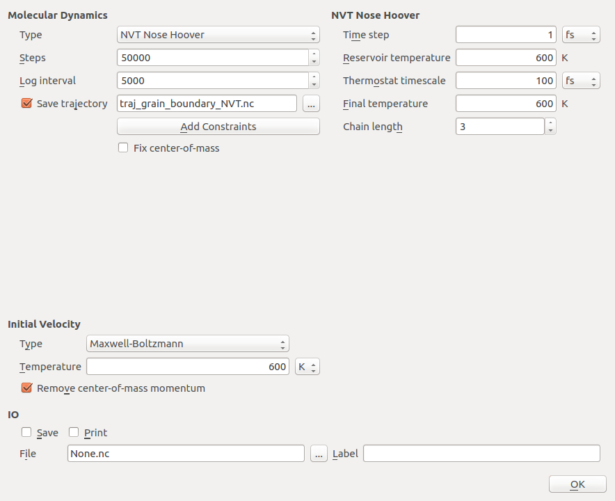
Select the Type as NVT Nose Hoover.
Set the number of steps to 50 000, and the log interval to 5000.
Choose a suitable trajectory filename, e.g.
traj_grain_boundary_equilibrate_NVT.nc.Select Maxwell-Boltzmann initial velocities at 600 K, and make sure that the center-of-mass removal box is checked.
Set the Reservoir temperature to 600 K, the final temperature will automatically change to 600K too. Leave the rest of the settings at default values.
Uncheck Save and Print and close the widget by clicking OK.
In the second MolecularDynamics block, the actual
non-equilibrium simulation will be set up. To do this:
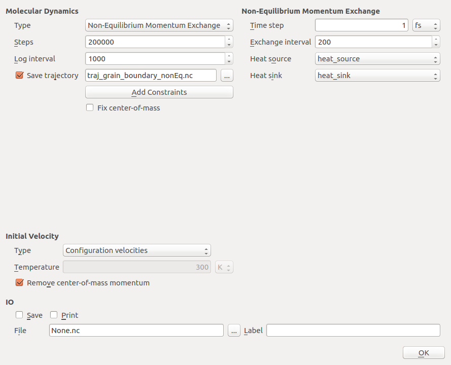
Select the type as Non-Equilibrium Momentum Exchange.
Set the number of steps to 200 000, and the log interval to 1000.
Select a suitable trajectory filename, e.g.
traj_grain_boundary_nonEq.nc.Set the initial velocities to ConfigurationVelocities, which means that the velocities stored in the configuration will be used.
Leave the Time step at the default value of 1 fs.
Set Exchange interval entry to 200, meaning that the exchange is triggered every 200 steps.
Uncheck Save and Print and close the widget by clicking OK.
Tip
Lowering the value of the Exchange interval entry will increase the transferred kinetic energy per simulation time, which causes a larger temperature gradient and a more distinct temperature profile. This will make the evaluation easier, but you generally should be careful with large temperature gradients, as their magnitude often by far exceeds the typical experimental temperature gradients.
Via the Heat source and Heat sink fields you can associate the tags, you have defined in the Builder, with heat source and sink, respectively. The final settings should look like the following.
Note
This simulation is set up for demonstration purposes to run reasonably fast - it should finish in about 10-15 minutes. For actual production simulations, you should use a larger (i.e. wider and much longer) system as well as a longer simulation time (e.g. 100 000 steps in the NVT equilibration and 800 000 steps or even more in the non-equilibrium simulation) to obtain reliable results and good statistics. As such NEMD simulations can be quite sensitive to finite size effects, you should always check your results for convergence with respect to system size and simulation time, if possible.
Run the entire simulation via the JobManager or save the script and run it at a terminal using atkpython.
Analyzing the results
After the simulations have completed, the trajectory files will appear on the LabFloor. Open the non-equilibrium trajectory in the Movie Tool and you will see that the average temperature remains constants during the entire simulation and the slab does not drift, as this would blur the temperature profile.
Investigating the interfacial thermal conductance
Open the same trajectory with the MD Analyzer plugin to investigate the thermal conductivity,
Select the Temperature profile button and click Load. It may take some time.
Attention
Here, you should carefully check the convergence of the temperature profile with respect to the simulation time. If you do not achieve a steady-state, you should run another non-equilibrium simulation with the same settings starting from the final snapshot of the previous one (in this case without the NVT equilibration).
To check whether the temperature profile has converged, you can compare the temperature profile between 1 and 50 ps, with that between 100 and 200 ps.
Tip
You can use the Add Line button to plot several curves on the same plot to make the comparison easier.
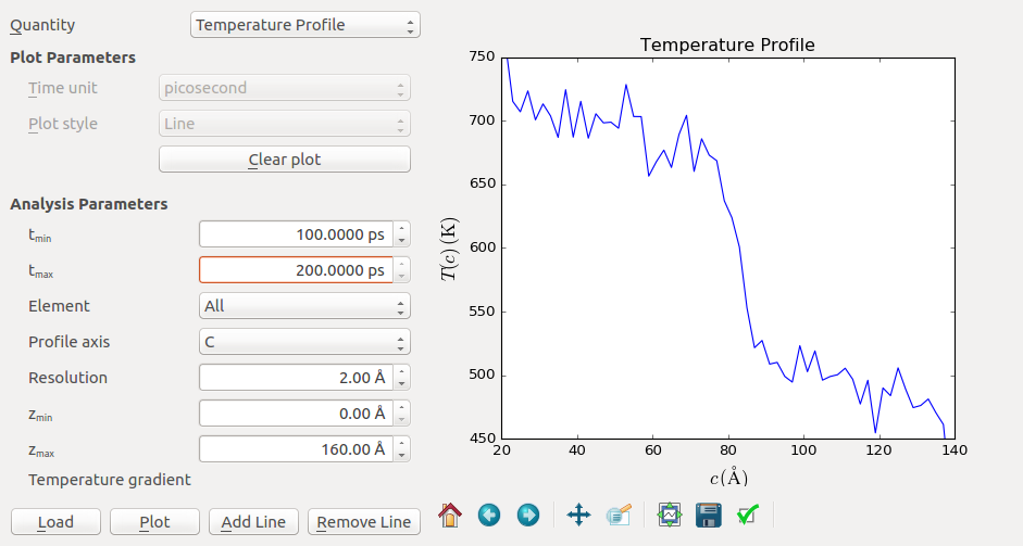
Use the zoom tool in the toolbar or the Edit plot button (on the bottom right) to zoom into the important features of the profile. Except for statistical fluctuations, your temperature profiles should be very similar to the plots shown here. In the plot below, the blue and green curve correspond to the intervals 1-50 ps and 100-200 ps, respectively.
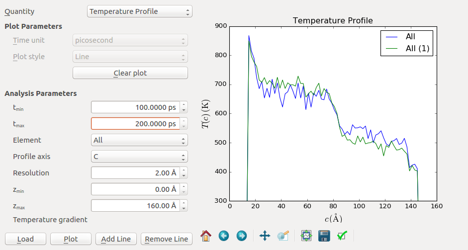
The temperature profile shows several typical features. First, a positive and a negative peak are visible at the beginning and end of the profile. These regions designate the heat source and sink, respectively. This non-linear part arises from the artificial transfer of kinetic energy due to the momentum exchange. You should always discard these regions in your analysis.
The next prominent feature is the temperature jump around z=80 Å. This is the interface region which provides additional thermal resistance. Let us take a closer look by zooming into this region (shown below for the 100-200 ps curve). Here it can be convenient to use the Edit plot button to set the minimum and maximum and both the x and y-axis.
The temperature jump connects around \(T_1 = 700\) K and \(T_2 = 500\) K, so the jump is about \(\Delta T = 200\) K. To calculate the Kapitza conductance you also need to know the average heat flux. This value can be read from the output at the bottom of the log file. In this example case, a value of \(\langle dQ/dt \rangle = 0.0010\) eV/fs is obtained. These values can then combined to calculate the Kapitza conductance by using the formula above.
As the units have to be converted correctly, the most convenient way to calculate this value is to use the built-in unit engine of QuantumATK.
Open the Editor and enter the following equation
dq_dt = 0.0010*eV/fs
delta_T = 200.0*Kelvin
G = dq_dt / delta_T
print("Kapitza conductance in Watt/Kelvin:  ",G.inUnitsOf(Joule/Second/Kelvin))
Run this script via the JobManager
(or atkpython) and save
it as kapitza.py. The log file will display the calculated Kapitza conductance in W/K. In this example, the result is 8 x 10 -10 W/K.
Investigating the grain size dependence of the thermal conductivity
You can also investigate the effect of the grain size, in this case modelled by the distance between the heat source or sink to the boundary, which is approximately 50 Å. Here, you will need to consider thermal conductivity instead of interfacial conductance. Use the MD Analyzer to extract the temperature gradient. Input reasonable numbers in \(Z_{min}\) and \(Z_{max}\) to select the linear region of the profile.
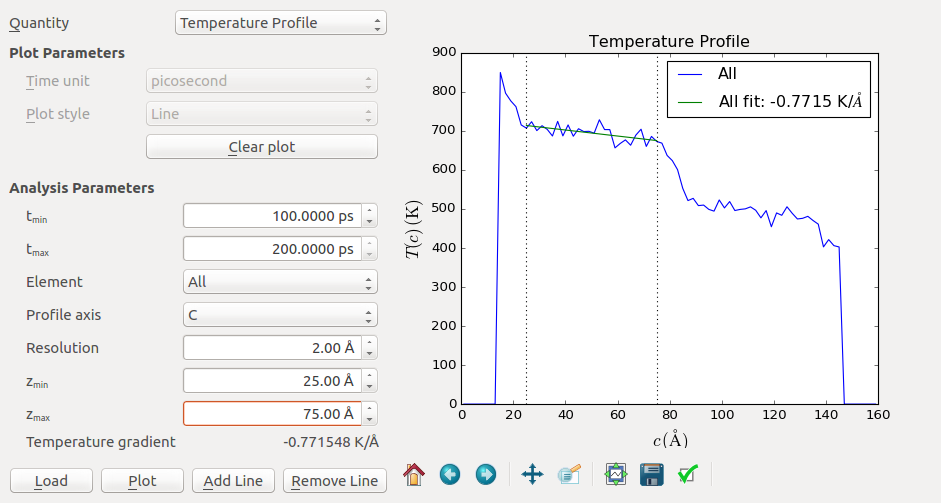
The program will automatically fit the slope and display the temperature gradient in the Parameters widget. A value of -0.77 K/Å is obtained for the (100) oriented grain in this example. You can repeat the procedure for the right grain and obtain a similar slope (around -0.90 K/Å). The slopes of the left and the right are unlikely to be identical, due to statistical fluctuations and different orientations.
We can now insert the calculated slope into the Fourier equation and,
together with the average transferred energy per time and the cross-sectional
area, calculate the thermal conductivity within the grain in a script.
The cross-sectional area A can be obtained from the A and B cell vectors.
You can find these by opening the
for the interface configuration in the Builder.
Open once again the kapitza.py and add the following lines in the bottom of
the script. You can repeat the lines to make a calculation for both the (100) and (110)
regions. When you have added the lines, send it to the Job Manager.
dq_dt = 0.0010*eV/fs
A = 11.46*11.24*Angstrom**2
dT_dz = 0.77*Kelvin/Angstrom
G = dq_dt / dT_dz / A
print("Grain conductivity in Watt/Kelvin/Meter:  ",G.inUnitsOf(Joule/Second/Kelvin/Meter))
The result for this example is 16.1 W/K/m for the (100) region. For the (110) oriented grain the conductivity amounts to 13.8 W/K/m. These values are considerably smaller than the simulated bulk thermal conductivity for silicon at 600 K, \(\kappa_{bulk}\) = 150 W/K/m, reported in Ref [3] using the same Stillinger-Weber potential. This behaviour is expected, since the thermal conductivity of a confined grain generally is lower than the corresponding bulk value [4]. This is due to the fact that the mean free path of the phonons is often much larger than 1 \(\mu m\), which means that the simulated grain size suppresses the thermal conductance [3][4].
To study the grain size dependence, you can repeat the simulation, preparing configurations with different lengths of the two crystal cells, as shown in Ref. [4].
The bulk conductivity can be obtained by performing several simulations at increasing grain sizes \(l\), plotting the inverse conductivity \(1/\kappa(l)\) over the inverse grain size \(1 / l\) and extrapolating to infinite grain sizes [3][4].
Non-equilibrium Green’s function method
In this section you will apply another method, the non-equilibrium Green’s function (NEGF) technique, to calculate the interface thermal conductance. You will use NEGF to calculate the phonon transmission spectrum and from that quantity obtain the thermal conductance. For more details about phonon transmission using the NEGF technique see e.g. Ref. [5] or the tutorial Thermoelectric effects in a CNT with isotope doping.
Preparing the configuration
For this method, we will set up a different calculation but the same interface
configuration.
Therefore, return to the Builder and select the interface
configuration you created earlier.
This time, before setting up the script, convert this configuration into a device configuration by clicking . Here you can leave all settings at default values and press OK.
Setting up the NEGF simulation
Send the device configuration to the
Script Generator by clicking the Send To icon
, and add 3 blocks:
- New Calculator
-

This will automatically add a DynamicalMatrix block as well.
Change the Default output file name to Silicon_grain_boundary_NEGF.nc, and
open the New Calculator block.
Select and the .
Uncheck and close the widget by clicking OK.
Open the OptimizeGeometry block and set the Force
tolerance to 0.001 eV / Å. The remaining parameters can
be left at their default values. Uncheck and
close the widget.
Next, open the PhononTransmissionSpectrum block and set the
q-point Sampling to Sampling and enter 12 for the sampling in both directions.
The settings should look like below
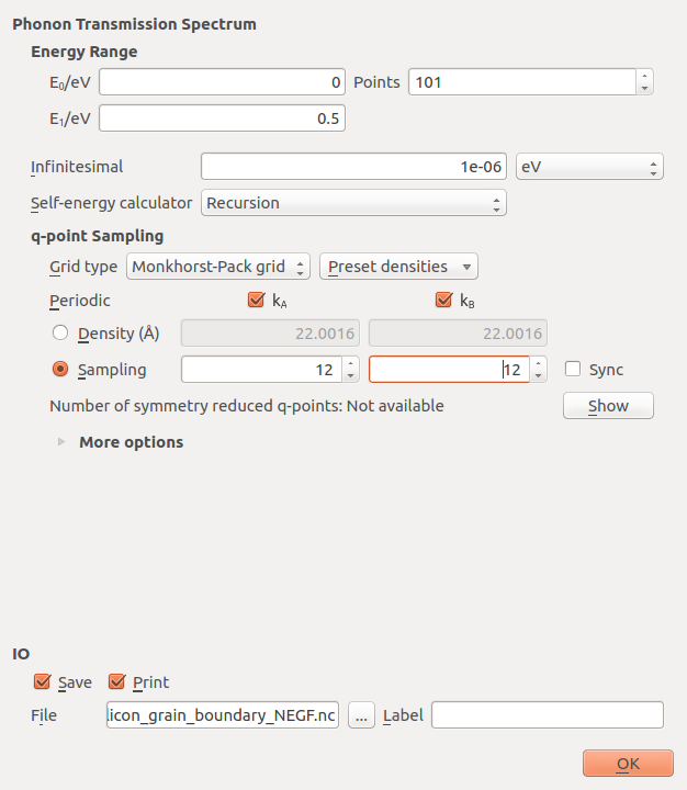
Click OK to close it. If you are running QuantumATK 2016.3 or earlier versions, then before running the script, you should make sure that Auto scan project files is unchecked under in the main QuantumATK window - this will prevent a slight bug form occuring during the simulation.
Then send the script to the JobManager . Save as
grain_boundary_NEGF.py when asked, and run it. The simulation should finish
in about 5-10 minutes.
Analyzing the results
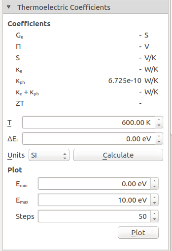
After the simulations have completed, the phonon transmission spectrum object will appear on the LabFloor. Select it and expand the Thermoelectric Coefficients plugin on the right-hand panel. To compare with the MD calculation of the thermal properties, set the temperature to 600 K and click Calculate. The thermal conductance should be printed in the window, and should be similar to the one shown below
Comparing results between RNEMD and NEGF
From the NEGF calculations we find a conductance of 6.7 x 10 -10 W/K, which is already quite close to the result calculated with RNEMD (which was 8 x 10 -10 W/K). The slight deviation can be attributed, among others, to the absence of inelastic phonon scattering in NEGF, and to finite size effects in our small model system, which affects in particular the particular the NEMD simulations.