Metadynamics Simulation of Cu Vacancy Diffusion on Cu(111) - Using PLUMED

Version: W-2024.09

In this tutorial you will learn how to setup and run metadynamics simulations in QuantumATK using the PlumedMetadynamics class and the PLUMED plugin. It will cover setting up a simulation to explore the free-energy landscape associated with the diffusion of a Cu vacancy on Cu(111), how to set up a metadynamics calculation, and how to analyze the results.

Introduction

Metadynamics [1] is a powerful method based on molecular dynamics to explore multidimensional free energy surfaces (FESs). It allows one to reconstruct the FES of a system as a function of a number of collective variables (CVs) which are based on the microscopic coordinates of the system.

In metadynamics, an additional bias potential is added to the system at regular intervals during the simulation time. This allows the system to escape deep free-energy minima and overcome high-energy barriers, thereby exploring efficiently the entire free-energy surface. Within materials science, the method has been used to investigate crystal polymorphism, solid-liquid interfaces, and chemical reactions in solids and surfaces. Here, you will apply it to investigate the diffusion of a Cu vacancy on Cu(111).

QuantumATK implements metadynamics via the PLUMED plugin. In this tutorial, we will introduce the method briefly, explain how to setup a metadynamics script for the vacancy diffusion on Cu(111), and how to analyze the resulting free-energy surface.

For more information on the metadynamics method, you may look at Refs. [2] and [3].

Theoretical Background

In metadynamics, an external bias potential is constructed in the phase space of a few selected degrees of freedom, $S$, generally called collective variables (CVs) [1]. $S$ is a set of $d$ functions of the microscopic coordinates $R$ of the system.

$$S(R) = (S_1 (R), ..., S_d (R)).$$

This potential is built as a sum of Gaussians deposited along the trajectory in the CVs space at time $t$. In its simplest version, the potential takes the form [2]

$$V(S,t) = \int_{0}^{t} dt^{'} \frac{W}{\tau} \exp\left( -\sum_{i=1}^{d} \frac{(S_i (R)-S_i({R}(t^{'} )))^2}{2\sigma_i^2} \right),$$

where $\tau$ is the Gaussian deposition stride, $\sigma_i$ is the width of the Gaussian for the $i$-th CV, and $W$ is the height of the Gaussian. The effect of the bias potential is to push the system away from local minima and allow it to visit new regions of the phase space.

Metadynamics Simulation of Cu Vacancy on Cu(111)

Creating a Vacancy on Cu(111)

To create the Cu vacancy on Cu(111), you first need to make a Cu(111) surface.

In the Builder, click on the in the Stash and select From Database. In the database dialog, ensure you are on the Crystals tab and search for Copper. Add ‘Copper’ to the Builder stash by double-clicking on the row. Next, find the Surface (Cleave) plugin in the plugins panel, either by using the filter or manually finding it under the Builders category. To create the Cu(111) surface, open the plugin and use the following settings:

1. Set the Miller indices to $\langle 1 1 1 \rangle$.

2. Set the surface indices to $v_1 = (4, 0)$ and $v_2 = (2, 4)$.

3. Set the out-of-plane cell vector as ‘Non-periodic and normal (slab)’, the thickness to six layers and the (top) vacuum gap to 10 Å.

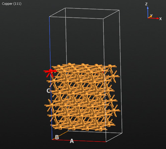
Next, create a vacancy by deleting the atom of the topmost layer with position $(x,y) = (0,0)$ (shown highlighted in the figure below):

Finally, find the Tags plugin (Selection Tools category) and select the 4 lower-most Cu(111) layers. Add a new tag by entering a name, ‘selection_0’ or another name of your choosing, and hitting Enter. A successfully added tag will show up in the list in the plugin and also be displayed in the tool-tip of any tagged atom. This tag will be used to fix them during the metadynamics simulation.

Now you are ready to create the workflow to perform the metadynamics simulation. Use the Send-to menu to send the structure to Workflows.

Creating the Metadynamics Workflow

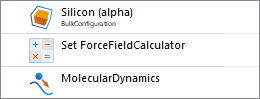
Sending the configuration automatically creates a new workflow with the name of the configuration, and the configuration itself added in a Configurations block. To set up the remainder of the workflow, add the following blocks:

• Calculators ‣ Set ForceFieldCalculator

• Optimization and Dynamics ‣ HookFunctions

• Optimization and Dynamics ‣ MolecularDynamics

Your workflow should now look like this:

Next, double-click on each of the added blocks to edit them:

1. In the Set ForceFieldCalculator block, ensure that the Potential set type is set to ‘Pre-defined potential set’. Find and select ‘EAM_Cu_2001b’ in the list of potential sets. To make it easier to find, use the search field to narrow down the list.

   

2. In the HookFunctions block, add a PlumedMetadynamics post-step hook. Click on the added row in the table to edit the hook settings. In the Script textbox, one can add any PLUMED [2] command. In this example we would like to add the following command:

   UNITS LENGTH=A TIME=fs ENERGY=96.48533645956869
   p: POSITION ATOM=81
   METAD ARG=p.x,p.y SIGMA=0.025,0.025 HEIGHT=0.05,0.05 PACE=1000 LABEL=restraint
   PRINT ARG=p.x,p.y,restraint.bias STRIDE=10 FILE=COLVAR
   

   

   There are four command lines:

   • UNITS: this line controls the units that will be used by PLUMED. Edit the lines as above, and the units of Å, femtoseconds, and eV will be used.

   • p: This line is used to define the atoms, whose cartesian position should be used as collective variable. In this case, the atom with index $81$.

     Note

     This value should be set according to the indexing used by PLUMED, where atom indexing starts from $1$, and not from $0$ as in QuantumATK. This value should therefore be set to “atom index $+ 1$”, where “atom index” is the index of the atom, which should be used in the collective variable.

   We will look at the potential energy surface in the $x$- and $y$- axis using the Gaussian function of the width ($0.025$) and height ($0.05$) on each axis.

   • METAD: This line controls the type of metadynamics and the shape of Gaussians functions that will be used during the simulations:

     • ARG: this flag is used to set the collective variables. In this case, we will use as collective variables the position of the atom $p$ along the Cartesian direction $x\ (p.x)$ and $y\ (p.y)$.

     • SIGMA: this flag is used to set the value of the width of the Gaussian functions $\sigma$ used for each collective variable. In this case, we will use $\sigma = 0.025$ for both collective variables.

     • HEIGHT: this flag is used to set the height of the Gaussian functions used for each collective variable. In this case, we will use a height of $0.05$ eV for both collective variables.

     • PACE: this flag is used to set the intervals at which a new Gaussian function will be added. In this case, we will add a new Gaussian function every $1000$ MD steps.

     • LABEL: this flag is used to set the name of the collective variables.

   • PRINT: This line controls the format of the PLUMED output.

     • ARG: this flag controls the variables that will be printed, in the present case $p.x$, $p.y$, and the bias.

     • STRIDE: this indicates the printing interval. In the present case, $10$ MD steps.

     • FILE: this line indicates the name of the output file.

   If you would like to know more detailed information, we recommend you to look in the PLUMED documentation. These commands are passed to the PlumedMetadynamics class. The latter is passed to the MolecularDynamics class using a hook function.

3. Open the MolecularDynamics block and set the simulation parameters on the two tabs as shown in the figures below. Also click on Add constraint and select for the previously added tag (by default, the tag is “selection_0”). Set the constraint type to FIXED.

   

For reference, the input files can be downloaded here:

• Worfklow Cu111_vacancy_hopping.hdf5

• Script Cu111_vacancy_hopping.py

Once you are done, send it to Jobs to run the simulation, which should take about 8 hours on 8 CPUs.

Analyzing the Results

In addition to the standard QuantumATK output, at the end of the job you will obtain the files COLVAR and HILLS. These two files are the output of PLUMED and will be used to analyze the metadynamics simulation.

To plot the profile of the free energy $\mathrm{F}$ as a function of the collective variables $\mathrm{CV\ 1}$ and $\mathrm{CV\ 2}$, you first have to run the script extract_F.py as atkpython extract_F.py. Three output files will be produced:

• F_vs_cv1.dat contains the data for $\mathrm{F}$ vs. $\mathrm{CV\ 1}$.

• F_vs_cv2.dat contains the data for $\mathrm{F}$ vs. $\mathrm{CV\ 2}$.

• F_vs_cv1_cv2.dat contains the data for $\mathrm{F}$ vs. $\mathrm{CV\ 1}$ and $\mathrm{CV\ 2}$.

The map of the free energy profile $\mathrm{F}$ can be obtained by running the script plot_F_vs_cv1_cv2.py as:

atkpython F_vs_cv1_cv2.py

The above plot shows a heat map of the free energy profile as a function of the collective variables $\mathrm{CV\ 1}$ and $\mathrm{CV\ 2}$. It can be seen that there are two minima on the free-energy surface, corresponding to the diffusion of the vacancy from one site to the neighboring one.

The evolution of the collective variables over the simulation time can be obtained by running the script cv1_cv2_vs_time.py as:

atkpython cv1_cv2_vs_time.py

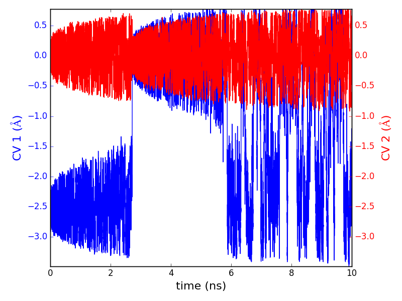
The resulting plot shows the evolution of $\mathrm{CV\ 1}$ (red) and $\mathrm{CV\ 2}$ (blue) as a function of the simulation time. It can be seen that $\mathrm{CV\ 2}$, which corresponds to the $y$ Cartesian coordinate, oscillates around a constant value ($\mathrm{CV\ 2}$ $= 0$ $\mathrm{Å}$), because both free energy minima occur at the same value of $y$. Conversely, the evolution of $\mathrm{CV\ 1}$, which corresponds to the x Cartesian coordinate, indicates that the simulation starts in the minimum on the left ($\mathrm{CV\ 1}$ $= -2.5$ $\mathrm{Å}$). The first minimum is filled until at approx. $2.2$ ns, and then the system moves to the second minimum ($\mathrm{CV\ 1}$$= 0$ $\mathrm{Å}$). After the second minimum is also filled, at around $6$ ns the system oscillates with equivalent probabilities between the two minima, until the simulation is completed.

The free energy barrier can also be analyzed by running the script barrier.py as:

atkpython barrier.py

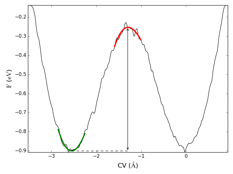
The results show that the barrier has a height of $0.647$ eV, in good agreement with the results in [4].

References

[1] (1,2)

Alessandro Laio and Michele Parrinello. Escaping free-energy minima. Proc. Natl. Acad. Sci., 99(20):12562–12566, 2002.

[2] (1,2,3)

Barducci, Alessandro and Bonomi, Massimiliano and Parrinello, Michele. Metadynamics. WIREs: Comput. Mol. Sci., 1(5):826–843, 2011. doi:10.1002/wcms.31.

[3]

Kristof M. Bal and Erik C. Neyts. Merging Metadynamics into Hyperdynamics: Accelerated Molecular Simulations Reaching Time Scales from Microseconds to Seconds. Journal of Chemical Theory and Computation, 11(10):4545–4554, 2015.

[4]

Suresh Kondati Natarajan and Jorg Behler. Self-Diffusion of Surface Defects at Copper-Water Interfaces. The Journal of Physical Chemistry C, 121(8):4368–4383, 2017.