How to Setup Basic Molecular Dynamics Simulations
Version: U-2022.12
In this tutorial, you will learn how to setup basic molecular dynamics (MD) simulations and analyze the resulting trajectories using the NanoLab GUI in QuantumATK ![]() . At the end of this tutorial, you will be familiar with simulating systems in a microcanonical ensemble (NVE), canonical ensemble (NVT) and isothermal-isobaric ensemble (NPT), using QuantumATK.
. At the end of this tutorial, you will be familiar with simulating systems in a microcanonical ensemble (NVE), canonical ensemble (NVT) and isothermal-isobaric ensemble (NPT), using QuantumATK.
Pre-requisites
Basic familiarity with NanoLab and atkpython
Basic familiarity with Molecular Dynamics simulations. If needed, you can read our technical note on Molecular Dynamics for a basic introduction to MD along with best practices, tips and tricks when setting up and analyzing MD simulations.

NVE Simulations
Let us setup a microcanonical ensemble simulation in which the number of particles (N), volume of the simulation cell (V) and energy of the system (E) remains constant. Import the geometry we will need, Silicon_bulk.py, to your Builder stash.
Workflow
Select the silicon supercell in Builder stash.
Click on the
 icon and send the bulk configuration to the Workflow Builder
In the Workflow Builder, change the output Filename at the bottom of the middle panel to
md-nve-1fs.hdf5.Add the following blocks to the Build panel by double clicking on the corresponding icons in the QuantumATK tab in the right-hand panel:
Under Calculators:
 Set ForceFieldCalculator
Under Optimization and Dynamics:
 MolecularDynamics
The resulting workflow will look like the below picture
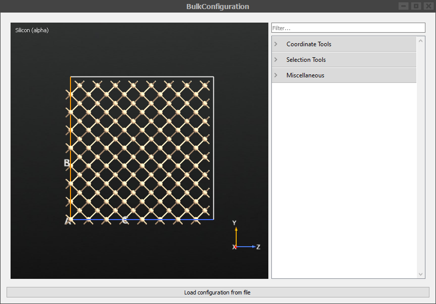
Double click the Silicon (alpha) block to visualize the bulk supercell. This is the system we will run MD for.
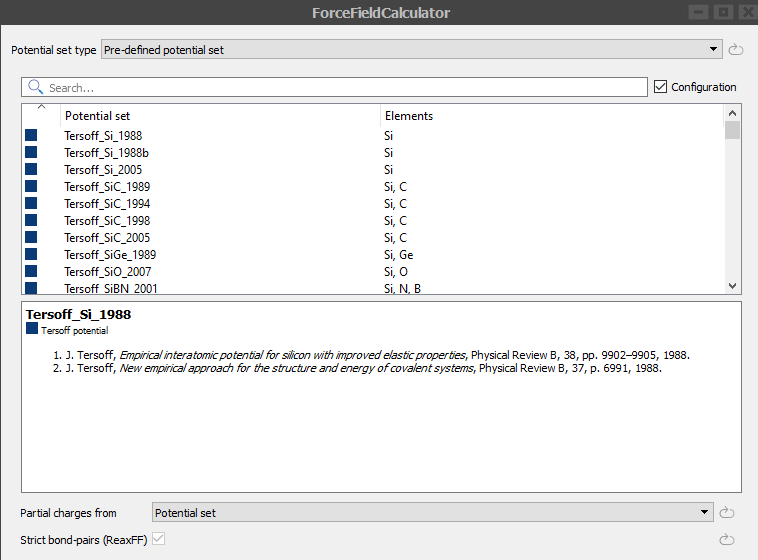
Double-click on the
Set ForceFieldCalculator block and select the Tersoff_Si_1988 parameter set as shown below
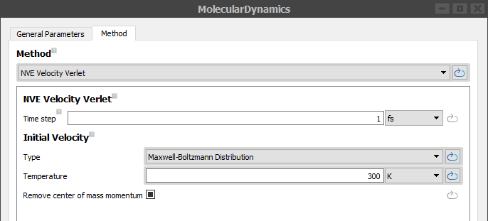
Double-click on the MolecularDynamics block, set the Steps to 1000, Log interval to 5 and set Fix the center of mass constraint
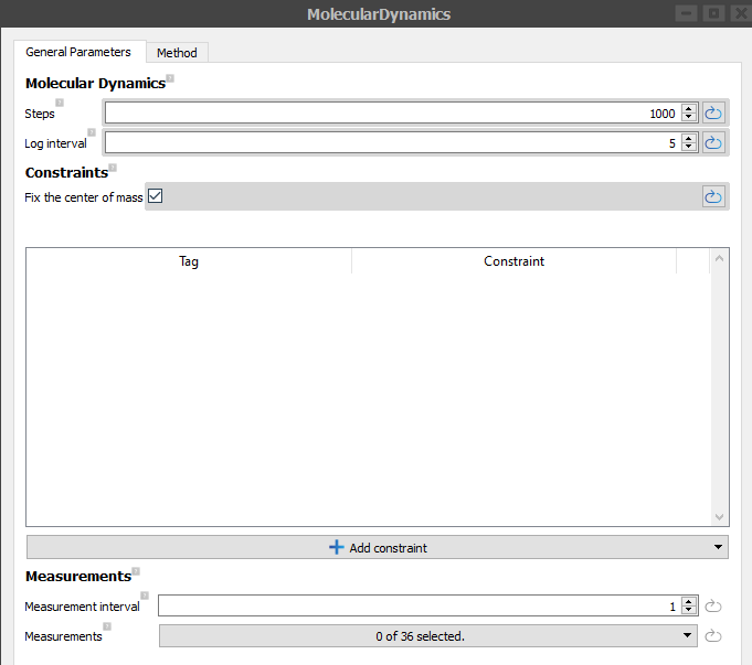
Go to Methods tab and choose Method as NVE Velocity Verlet from the pull down menu, set Initial velocity Type to Maxwell-Boltzmann Distribution and Temperature to 300 K.
Send the workflow to the Job Manager as a script using
and save the script as md-nve-1fs.py. This script runs in a few seconds, it can run locally.
Alternatively, download the workflow md_tutorial_nve_1fs.hdf5 to your project folder, open it in the Workflow Builder Tool in the Nanolab, export to script and submit the job.
Analyzing the Results
Once the simulation is finished, select the md-nve-1fs.hdf5 file from the project folder and double-click the MDTrajectory_0 object from the Data View. The trajectory will open in the Movie Tool plugin. Using the Movie Tool plugin, you can investigate the temperature as well as the kinetic, potential, and total energies of the system as a function of simulation time. Simultaneously, an animation of the motion of the atoms is displayed.

If you take a look at the temperature, you will observe the temperature dropping immediately and then oscillate around the set temperature. The reason is that the displayed temperature is the instantaneous temperature of the system, calculated from the kinetic energy of the atoms, via \(E_{kin}(t) = 3/2 N k_B T(t)\). Since the atoms are not free but interact with the neighboring atoms in the lattice, their initial kinetic energy will be partially converted into potential energy. For an NVE ensemble, a crucial parameter to monitor is the conservation of the total energy and find that the total energy curve in the Movie Tool remains constant with only small oscillations which are acceptable.
Tip
Try changing some MD parameters and see how they affect dynamics. For more tips, refer to Molecular Dynamics.
NVT Simulations
In NVT, we keep the temperature constant instead of the energy as in the NVE case. Download the workflow md_tutorial_nvt_300k.hdf5 to your project folder and open it in the Workflow Builder Tool in the Nanolab.
Workflow
The workflow should look similar to the NVE case, but the MolecularDynamics block should list NVT as the MD method and a reservoir temperature of 300 K will be listed. In this example, we use the Nose-Hoover type thermostat coupling to the reservoir. For more details on this method and other available thermostats, refer to the technical note on Molecular Dynamics.
After loading the workflow, export it as a script and submit the job.
Analyzing the Results
After the simulation is completed, open the NVT MD trajectory object with the Movie Tool and take a look at the temperature curve.
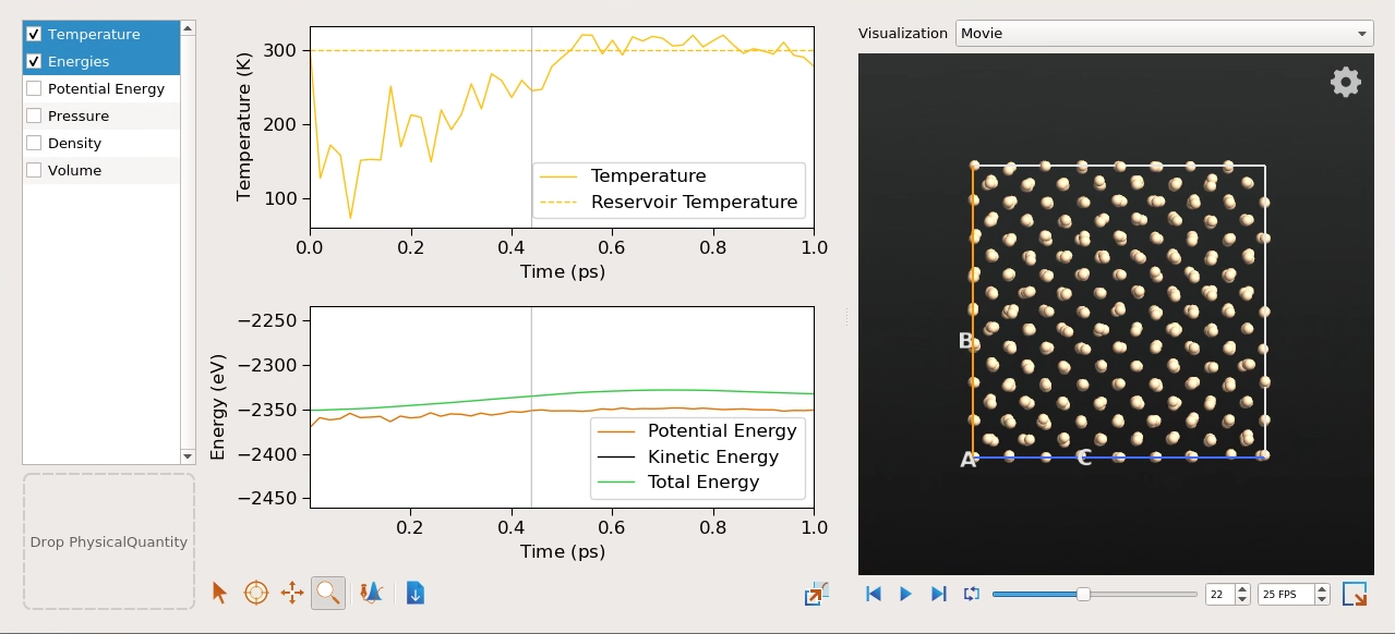
You will find that after a short initial equilibration period the curve fluctuates slightly around the selected reservoir temperature of 300 K. In fact, it does not look very different from the results of the NVE simulation in the previous section. In contrast to the NVE simulation, however, the final equilibrium temperature of the system is independent of the initial value, set via the Maxwell-Boltzmann distribution, and is instead coupled to the reservoir temperature. Let us take a closer look at this now.
Download the workflow md_tutorial_nvt_1000k.hdf5 in which the reservoir temperature is set to 1000 K.
Leave the initial velocities as a Maxwell-Boltzmann distribution at 300 K and run the script.
On opening the resulting trajectory in the movie tool, we see the temperature curve starting at an initial value of 300 K (as selected via the Maxwell-Boltzmann distribution).
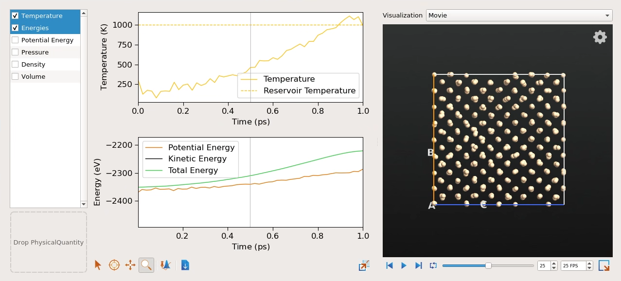
Subsequently, as the system is in contact with the heat bath, the temperature quickly increases towards the reservoir temperature of 1000 K. You may also notice an increase in the total energy. In contrast to NVE simulations, this is not a sign of poorly chosen parameters, but reflects the fact that energy is exchanged with the virtual heat bath.
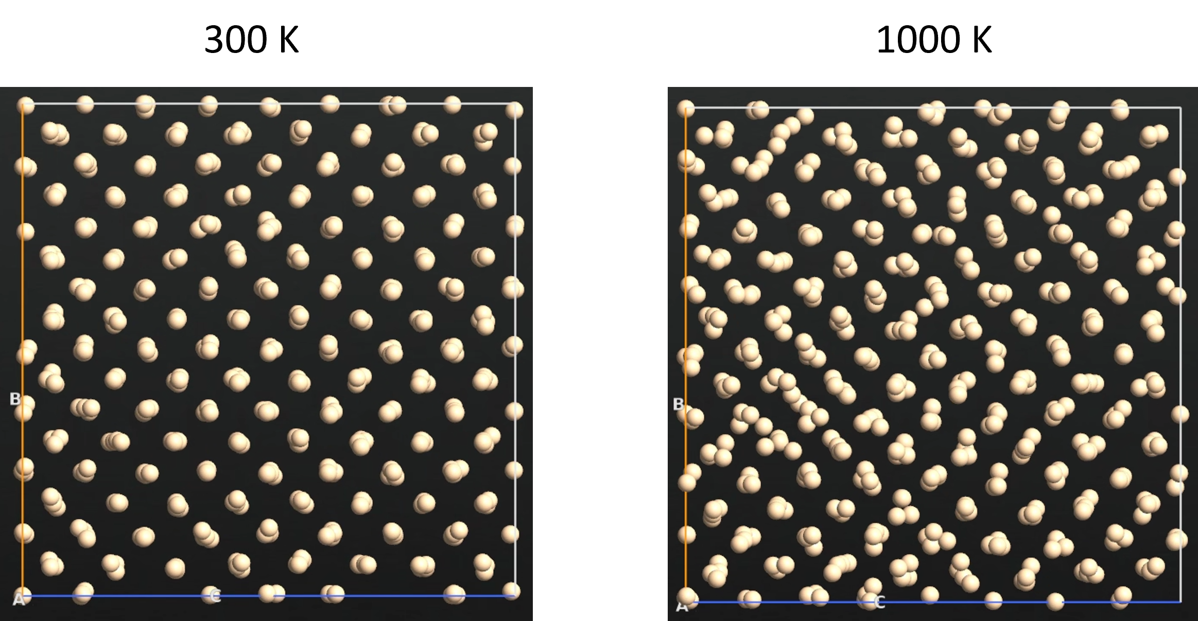
During the simulation at 1000 K, the motion of the atoms increases compared to the previous simulation at 300 K.
If you increase the reservoir temperature to even higher values (e.g 3000 K), you will find that the crystal will begin to melt and become partially amorphous. Annealing crystals at high temperatures is in fact a common way to generate amorphous structures of a material. You can learn more about this method in the tutorial Generating Amorphous Structures.
Warning
Setting too high a temperature on a minimum energy configuration might result in the generation of very large forces on the atoms which could destabilize the system. Instead, slowly heat up the system from room temperature using a suitable heating rate.
NPT Simulations
In this ensemble, we keep the number of particles, pressure and temperature constant.
Download the workflow md_tutorial_npt_300k_1bar.hdf5 to your project folder and open it in the Workflow Builder tool in the NanoLab.
Workflow
The main difference you will observe in the MD block is the choice of NPT method. We use NPT Martyna Tobias Klein barostat in this example. For more details about this method and other NPT methods, refer to Molecular Dynamics. As you will notice the reservoir temperature and pressure are set to 300 K and 1 bar, respectively and an isotropic coupling is selected. This is because are simulating the system at standard temperature and pressure conditions and also allow the system to relax equally on all three lattice directions. Anisotropic coupling can be enabled to choose to fix some simulation cell boundaries.
Export the workflow as script and submit the job.
Analyzing the Results
Opening the trajectory with the Movie Tool, you can monitor the changes in the size and shape of the cell during the simulation. The temperature fluctuates around the selected reservoir temperature of 300 K.

To inspect the volume fluctuations you can select the volume measurement in the Movie Tool. The cell volume will show pronounced oscillations. These oscillations are a typical outcome of the Nose-Hoover-like temperature and pressure control. As long as their magnitude stays within reasonable boundaries, and does not increase dramatically throughout the simulation, there is no need to worry. The period of these oscillations can be changed by the Barostat timescale setting. The amplitude and frequency of the oscillations increases with decreasing barostat timescale.
The pressure during the simulation, seen by selecting the Pressure measurement in the Movie Tool, shows a similar behavior. It oscillates around the target pressure of 1 bar, but the amplitude is large. Such large fluctuations of the instantaneous pressure values are in fact not unusual in MD simulations, as the pressure is calculated based on the stress, which varies considerably with small changes of the volume. Moreover, pressure is a macroscopic property, and for such a small system it is more reasonable to consider the corresponding average rather than the instantaneous values.
Conclusion
You have learnt how to use the Workflow Builder tool to set up basic molecular dynamics simulations of NVE, NVT and NPT ensembles. You also know how to view the resulting trajectories using the Movie tool and interpret the results.
Feel free to change the MD settings and run the simulations to see how the dynamics changes and to familiarize yourself with the method.
You can try adding multiple MD blocks within a workflow to simulate the system in different ensembles in a sequential manner. For more inspiration, checkout predefined MD templates in the Templates section of the Workflow Builder.