Introduction to noncollinear spin
Version: 2016.3
In standard (collinear) spin-polarized calculations, the spin quantum number (up or down) is added to the electronic states. In contrast, noncollinear spin allows the electronic spin to point in any direction. This introduces a few more concepts – and possibilities! – which may be somewhat unfamiliar. This tutorial therefore provides a simple introduction to ATK-DFT calculations with noncollinear spin densities.
As briefly stated above, noncollinear magnetism refers to situations where the spin direction depends on position in such a way that there is no particular direction in which all the spins are (anti)parallel. Noncollinear spins are quite ubiquitous in nature, and include systems with spin spirals (e.g. chromium) and helicoids, canted spins (e.g. manganites), and most commonly domain walls in ferromagnetic materials. ATK allows you to study systems with noncollinear spins from first principles, but it is technically and conceptually quite different from the familiar case of collinear spin.
From collinear to noncollinear spin
It is important to realize that the familiar concept of spin as being either up or down – and all derived quantities also being labeled by this quantum number – does not work in a noncollinear DFT calculation. Instead, the eigenstate of an atom is a spinor with a certain mixing of both spin up and down channels, and many quantities – like the electron transmission spectrum – become a 2x2 matrix rather than two separate numbers (spin up and down transmission).
Another important aspect of noncollinear calculations in practice is that they require in general more CPU time and memory than the corresponding spin-polarized or unpolarized calculation. SCF convergence may also be harder to achieve, since the electronic states have more degrees of freedom.
Two key features have therefore been implemented in QuantumATK to improve the SCF convergence rate for noncollinear calculations:
use of a collinear spin-polarized calculation as starting point;
a special density mixing scheme which diagonalizes the density matrix before mixing it.
Using these techniques, the required number of iterations to reach the selfconsistent noncollinear ground state can be reduced substantially.
Getting started
As mentioned above, the recommended approach for noncollinear calculations is to use a collinear spin-polarized calculation as the initial state. This tutorial therefore takes as starting point the collinear spin-parallel ground state of a simple carbon-chain device obtained in the tutorial Transmission spectrum of a spin-polarized atomic chain.
Start by opening QuantumATK and create a new project. If you have not already
completed the aforementioned tutorial, use a script to calculate the
required spin-parallel ground state: carbon_para.py. The calculation takes
less than 5 minutes and saves the result in the file carbon_para.nc.
You will now use the selfconsistent calculation stored in this file as the starting point for a noncollinear calculation of the same linear 1D chain of carbon atoms. However, instead of just considering the parallel and anti-parallel (left electrode up, right electrode down) spin configurations, you will consider any angle of spin rotation between the two electrodes.
Spin rotation of 120°
Open the QuantumATK  Editor (or your own favorite editor) and
copy/paste the following lines of ATK Python code
into it:
Editor (or your own favorite editor) and
copy/paste the following lines of ATK Python code
into it:
 1# Read in the collinear calculation
 2device_configuration = nlread('carbon_para.nc', DeviceConfiguration)[0]
 3
 4# Use the special noncollinear mixing scheme
 5iteration_control_parameters = IterationControlParameters(
 6    algorithm=PulayMixer(noncollinear_mixing=True)
 7    )
 8
 9# Get the calculator and modify it for noncollinear LDA
10calculator = device_configuration.calculator()
11calculator = calculator(
12    exchange_correlation=NCLDA.PZ,
13    iteration_control_parameters=iteration_control_parameters
14    )
15
16# Define the spin rotation
17theta = 120*Degrees
18left_spins   = [(i, 1, 0*Degrees, 0*Degrees) for i in range(3)]
19center_spins = [(i+3, 1, theta*i/5, 0*Degrees) for i in range(6)]
20right_spins  = [(i+9, 1, theta, 0*Degrees) for i in range(3)]
21spin_list    = left_spins + center_spins + right_spins
22initial_spin = InitialSpin(scaled_spins=spin_list)
23
24# Setup the initial state as a rotated collinear state
25device_configuration.setCalculator(
26    calculator,
27    initial_spin=initial_spin,
28    initial_state=device_configuration
29    )
30
31# Calculate and save
32device_configuration.update()
33nlsave('carbon_nc120_ncmix.nc', device_configuration)
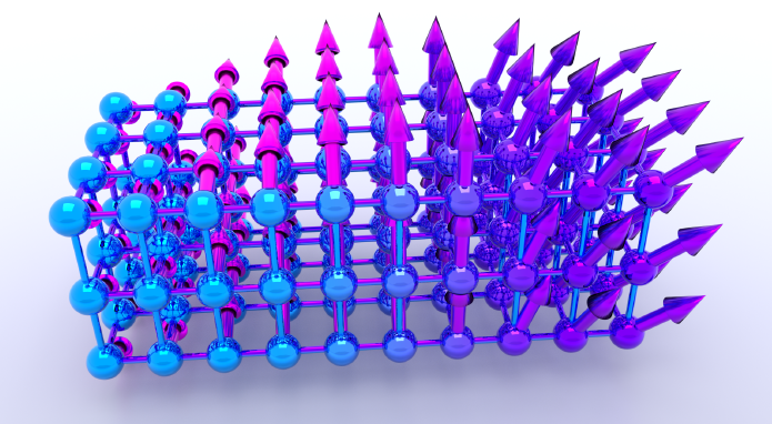
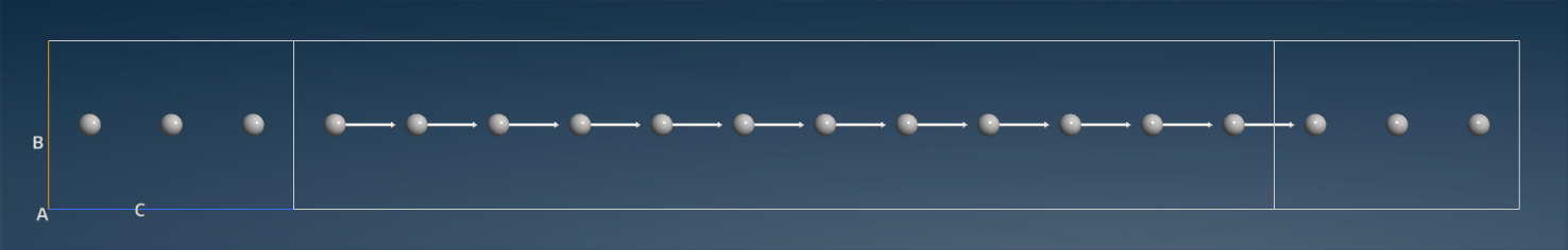
The spin setup corresponds to the spin polarization of the atoms in the left electrode pointing along the transport axis C, while in the right electrode the polarization is rotated 120 degrees (polar angle in a coordinate system where the XY plane is the equator). In the central region, the angle is interpolated between these two values. Note that this is just the initial spin configuration – the actual spin polarization vectors will be computed selfconsistently and may therefore change (you can see the result below).
Note
The initial electrode spins are automatically identical to the initial spins on the atoms in the “electrode extensions” in the central region, in this case the 3 first and last atoms.
Save the script as carbon_nc120.py, and then run it – it should
take a few minutes only. Remember that you can use the  Job Manager for this.
Analysis
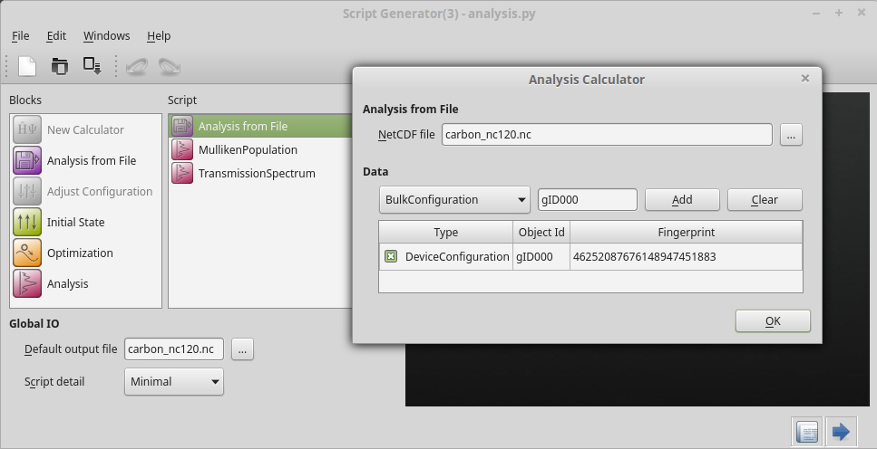
The NEGF calculation is done, and it’s time to do some analysis. Use the Script Generator to set up the post-SCF analysis calculations:
Open the
 Script Generator.
Double-click the
 Analysis from File
block to insert it into the Script panel. Then double-click the
inserted block and select the file
Analysis from File
block to insert it into the Script panel. Then double-click the
inserted block and select the file carbon_nc120.nc, which was generated in the previous section.Add a
 MullikenPopulation analysis block.
Add a
TransmissionSpectrum analysis block
(use default parameters).Set the output file to
carbon_nc120.nc.Run the script using the
Job Manager.
The analysis script should look roughly like this:
 1# -*- coding: utf-8 -*-
 2# -------------------------------------------------------------
 3# Analysis from File
 4# -------------------------------------------------------------
 5path = u'carbon_nc120.nc'
 6configuration = nlread(path, object_id='gID000')[0]
 7
 8# -------------------------------------------------------------
 9# Mulliken Population
10# -------------------------------------------------------------
11mulliken_population = MullikenPopulation(configuration)
12nlsave('carbon_nc120.nc', mulliken_population)
13nlprint(mulliken_population)
14
15# -------------------------------------------------------------
16# Transmission Spectrum
17# -------------------------------------------------------------
18kpoint_grid = MonkhorstPackGrid()
19
20transmission_spectrum = TransmissionSpectrum(
21    configuration=configuration,
22    energies=numpy.linspace(-2,2,101)*eV,
23    kpoints=kpoint_grid,
24    energy_zero_parameter=AverageFermiLevel,
25    infinitesimal=1e-06*eV,
26    self_energy_calculator=RecursionSelfEnergy(),
27    )
28nlsave('carbon_nc120.nc', transmission_spectrum)
29nlprint(transmission_spectrum)
Mulliken populations
The Mulliken populations is now available as an analysis object on the QuantumATK LabFloor, and can be inspected using the Text Representation tool in the right-hand panel bar.
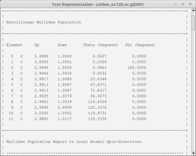
You immediately notice the difference to the collinear case: Now the
Mulliken population on each atom is described by 4 variables; Up,
Down, Theta and Phi. Note that Phi=180 is equivalent to Phi=0.
The sum of the up and down populations
corresponds, as usual, to the total Mulliken charge (the number of electrons),
and their difference – combined with the two angles – forms a spin
polarization vector, which can be visualized in the QuantumATK  Viewer:
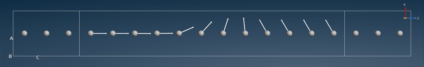
It is clear that the spin polarization direction changes smoothly between the two values in the electrodes.
Tip
The Viewer view plane used in the image is ZX. Use the Camera settings menu to select a view plane different from the default ZY.
Transmission spectrum
The TransmissionSpectrum analysis object is also available
on the LabFloor. Use the Text Representation tool to inspect it –
you again see that it has 4 components; up, down, real-up-down
and imag-up-down:

The last spin component (imag-up-down) is very small in this simple system, but will in general be important in cases where the spins have other directions.
Note
Any quantitty calculated using noncollinear spin is represented as a 2x2 matrix (a spinor) with different mixing of up and down components: \(\uparrow \uparrow\), \(\downarrow \downarrow\), \(\uparrow \downarrow\), and \(\downarrow \uparrow\).
As explained in the QuantumATK Manual section Spin, a range of different spin projections may be derived from these 4 basic components, including Sum, X, Y, and Z:
Use the Transmission Analyzer plugin to plot the transmission spectrum. The transmission components Sum, X, Y, and Z are by default included in the graph:
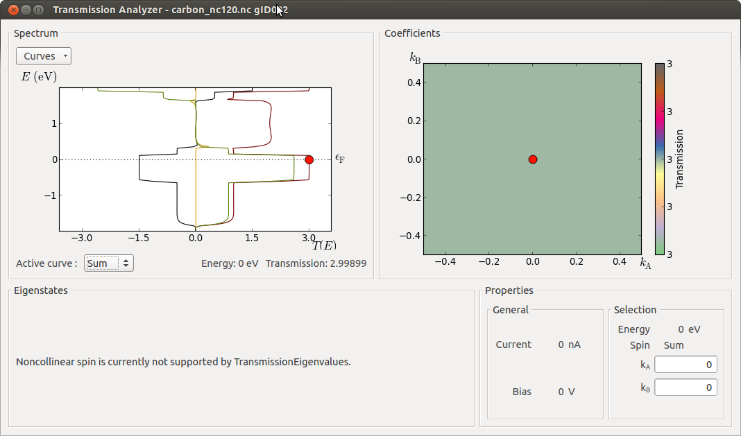
Tip
The drop-down menu Curves at the top-left of the window lets you choose which spin projection to include, while the lower “Active curve” option is for choosing which k-point resolved spectrum to show in the right-hand “Coefficients” plot (for this 1D system there is only one transmission coefficient, at (\(k_A\), \(k_B\))=(0,0), so the plot is rather uninteresting). This can also be chosen by clicking the corresponding transmission curve.
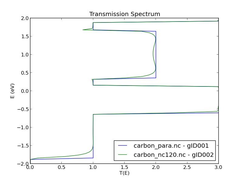
The Spin.Sum transmission spectrum is very similar to the parallel collinear case, and very different from the anti-parallel collinear case. This may surprise, since the spin configuration in the electrodes are more anti-parallel than parallel. However, due to the noncollinear degrees of freedom, the electron can propagate in a helical state when moving from left to right, and this allows for a high transmission. In fact, if you set the rotation angle to 180 degrees, corresponding to anti-parallel alignment of the electrodes, the result will be almost the same.
The figure below compares the transmission spectra for the collinear spin-parallel state and the noncollinear state, using the Compare Data plugin.
Spin-orbit interactions
Spin-orbit coupling (SOC) is most often neglected in electronic structure calculations, but it can actually be included in a noncollinear calculation, provided that suitable pseudopotentials are used. You can find more details in the tutorial Spin-orbit splitting of semiconductor band structures.
The carbon chain considered here has a very small SOC, so results with spin-orbit interactions included in the electronic structure method will hardly be different from those obtained above. Even so, if you wish to include SOC in calculations similar to the ones outlined in the section Spin rotation of 120°, simply change the exchange–correlation method and pseudopotentials used in the ATK-DFT calculator:
use spin-orbit GGA (SOGGA) exchange–correlation and SG15-SO pseudopotentials,
or use spin-orbit LDA (SOLDA) exchange–correlation and OMX pseudopotentials.
Spin-orbit GGA
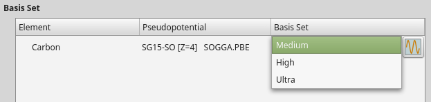
When setting up the initial collinear calculation, saved as carbon_para.nc,
choose SGGA exchange-corerlation instead of LSDA, and navigate to the
Basis set/exchange correlation calculator settings and select the SG15-SO
type pseudopotential. You will usually have the option to choose between
three different basis set sizes:
Note
The density mesh cutoff should not be smaller than 100 Ha when using SG15 pseudopotentials.
Run the spin-polarized GGA calculation, which creates carbon_para.nc,
and then use SOGGA.PBE exchange-correlation when setting up the
calculator with spin-orbit coupling:
 1# Read in the collinear calculation
 2device_configuration = nlread('carbon_para.nc', DeviceConfiguration)[0]
 3
 4# Use the special noncollinear mixing scheme
 5iteration_control_parameters = IterationControlParameters(
 6    algorithm=PulayMixer(noncollinear_mixing=True)
 7    )
 8
 9# Get the calculator and modify it for spin-orbit GGA:
10calculator = device_configuration.calculator()
11calculator = calculator(
12    exchange_correlation=SOGGA.PBE,
13    iteration_control_parameters=iteration_control_parameters
14    )
Spin-orbit LDA
When setting up the initial collinear calculation, saved as carbon_para.nc,
navigate to the Basis set/exchange correlation calculator settings
and select the OMX type pseudopotential.
You will usually have the option to choose between different basis set sizes:
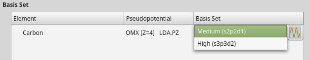
Note
The OMX potentials are in general fairly “hard”, so they often require a larger mesh cutoff than e.g. the FHI potentials, usually at least 150 Ha.
Run the spin-polarized LDA calculation, which creates carbon_para.nc,
and then use SOLDA.PZ exchange-correlation when setting up the
calculator with spin-orbit coupling:
 1# Read in the collinear calculation
 2device_configuration = nlread('carbon_para.nc', DeviceConfiguration)[0]
 3
 4# Use the special noncollinear mixing scheme
 5iteration_control_parameters = IterationControlParameters(
 6    algorithm=PulayMixer(noncollinear_mixing=True)
 7    )
 8
 9# Get the calculator and modify it for spin-orbit GGA:
10calculator = device_configuration.calculator()
11calculator = calculator(
12    exchange_correlation=SOLDA.PZ,
13    iteration_control_parameters=iteration_control_parameters
14    )
Tip
What’s next? You should consider the tutorial Noncollinear calculations for metallic nanowires.
Noncollinear spin is essential when computing the spin transfer torque, see for example the tutorials Spin Transfer Torque and Spin transport in magnetic tunnel junctions.
The tutorials Spin-orbit splitting of semiconductor band structures and Relativistic effects in bulk gold give more details of spin-orbit calculations with ATK-DFT.