Modeling Vacancy Diffusion in Si0.5 Ge0.5 with AKMC
Version: 2017
In this tutorial, we will model vacancy diffusion in a Si0.5 Ge0.5 alloy using the Adaptive Kinetic Monte Carlo method (AKMC). AKMC is an algorithm for performing Kinetic Monte Carlo (KMC) simulations on-the-fly without having to have a predefined set of states and reaction mechanisms. The reaction mechanisms are determined by locating saddle points on the potential energy surface and then using Harmonic Transition State Theory (HTST) to calculate the reaction rate. You can learn more about the AKMC method in this tutorial: Adaptive Kinetic Monte Carlo Simulation of Pt on Pt(100).
Note
For typical MD simulations, it is impractical to model more than a couple of hundred nanoseconds. However, by using AKMC, we will be able to model the dynamics of the system on a longer time scale. This is because the KMC simulation describes the dynamics of the system as transitions between states that – once found – can be computed very quickly.

Obtaining an Initial Structure
In order to generate the initial Si0.5 Ge0.5 alloy structure,
we will use the in the
 Builder, implemented in the ATK 2015 version. If you have an
older version, you can use this script instead:
Builder, implemented in the ATK 2015 version. If you have an
older version, you can use this script instead: initial-structure.py.
Open the
Builder.Using , add the Silicon (alpha).
Click the , set A = 4, B = 4, C = 4, and press the Apply button.
Select the .
Use the default to substitute 50 percent of Si with Ge.
Click the Create button.
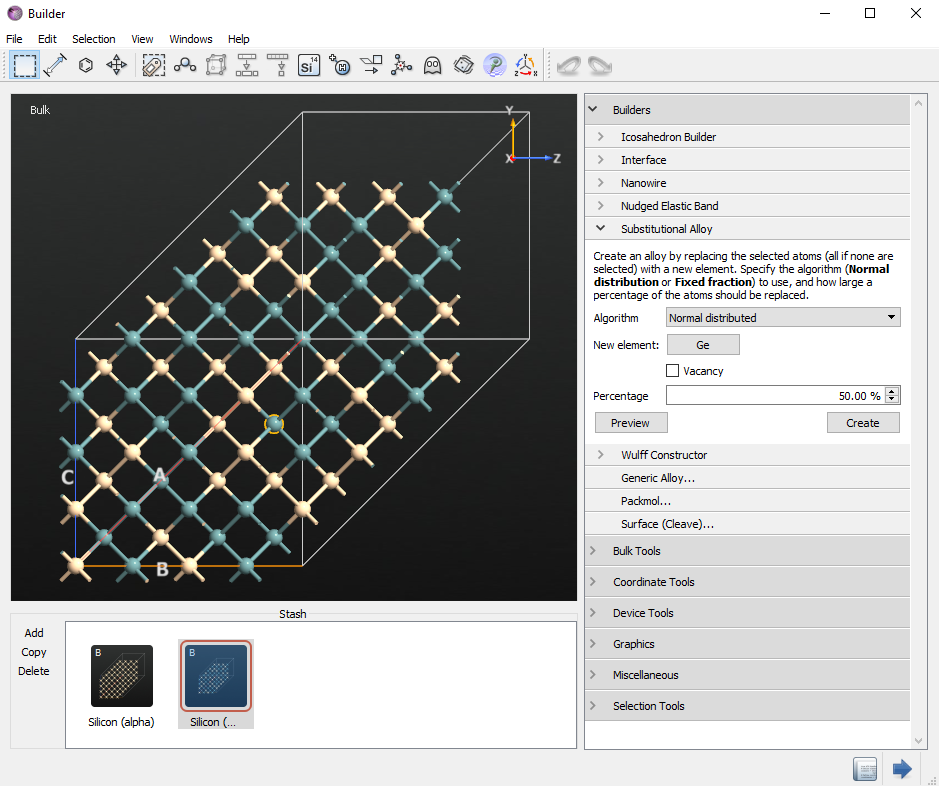
You now see the initial alloy in the main window of the Builder and in the Stash. It might be different from the one shown here, as the alloy is randomly created. We make one Si vacancy in the initial structure. In this case, we delete one yellowish Si behind blue-colored Ge at the front site. You can make one Si vacancy randomly.
Now we will optimize the initial structure.
Send the initial configuration to the Script Generator by clicking the
 button.
Add
 New Calculator and
  OptimizeGeometry blocks.
Change the output name to
alloy.hdf5.Double-click the
New Calculator block and select the ATK-Classical calculator and choose the StillingerWeber_SiGe_1995 Parameter set.In the
OptimizeGeometry block, set the Force tolerance to 0.01 eV/Å.Send the script to the Job manager by clicking the
button.
You can also download and use the script initial-structure.py.
This script generates a silicon supercell and then randomly replaces Si atoms
with Ge atoms in order to achieve a 50:50 ratio and then creates a Si vacancy as shown below.
Run the script either by dragging it from the main QuantumATK window and dropping
it on the  Job Manager, or directly through the terminal.
Now you have generated a 4x4x4 supercell of SiGe with one vacancy, calculated
the optimized geometry and saved the structure to alloy.hdf5.
Note that this is a very small system, useful only for illustrative purposes.
You will need a larger system for scientifically valid modelling.
You can visualize the structure in QuantumATK by selecting the gID0001 object
from the alloy in the LabFloor and drag and drop it on the  Viewer.
The result is shown below.
Viewer.
The result is shown below.
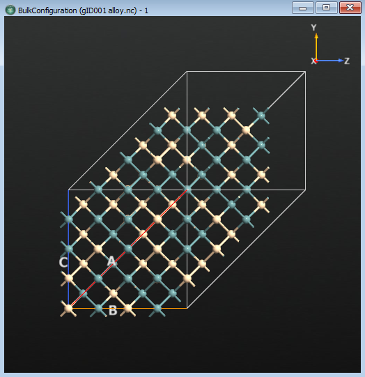
There is a vacancy in the structure, but it is difficult to see. You will perform a LocalStructure calculation to see which atoms do not have the typical diamond-like packing.
1. Drag the gID0001 object from the LabFloor to the
 Scripter.
2. In the Scripter, double click on .
3. Choose the default output file to be
Scripter.
2. In the Scripter, double click on .
3. Choose the default output file to be local_structure.hdf5.
4. Send the script to the Job Manager using the button and run the calculation. It should take no more than a minute.
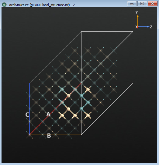
Now you can get a better look at the structure around the vacancies. From the main window, open the LocalStructure item in the Viewer and expand the Local Structure panel in the sidebar. Select Diamond-like. Now all of the atoms that are not near the vacancies, and thus have the ideal crystal structure, have been selected. Open the Properties dialog and in the Atoms tab and change the opacity to 0.1 for the selected atoms. This will highlight the atoms near the vacancies, by making the others almost transparent. The result is shown in the figure below. Note the obvious vacancy in middle of the cluster.
Running the AKMC Simulation
Now that you have an optimized initial structure, you can run the AKMC simulation.
Drag alloy.hdf5 from the main QuantumATK window to the Script Generator.
The New calculator will be automatically loaded in the Scripter. Starting from ATK 2017, AdaptiveKineticMonteCarlo is implemented in the Scripter. If you have an older version, you can download the script adding-akmc.py and append the contents in the  Editor instead of following the steps below.
Add the block.
Double click
AdaptiveKineticMonteCarlo.In the Saddle Search section, set the Number of searches to 100.
Go to the Optimization section, and press the Atomic Constraint Editor button.
Select one atom as far away as possible from the vacancy
Press the Add tag from Selection button
Change from None to Fixed for Constraint.
Press the OK button.
In the Molecular Dynamics part, set the temperature to 1200 K.
Note
If you look at the Help… button on the AdaptiveKineticMonteCarlo widget, settings and definitions are introduced in detail. Higher number of searches and higher confidence give us more accuracy, but is also computationally more expensive.
Save the output file as
akmc.hdf5.
Tip
When you see the AKMC script (either from the Scripter or in adding-akmc.py), it enables a restart of the simulation, by reusing the
existing files if they exist. For a detailed description of the parameters for
the AKMC object, please see the tutorial:
Adaptive Kinetic Monte Carlo Simulation of Pt on Pt(100).
Now run the script. Running the script should take no more than half an hour
on a desktop machine. At the end, you will have a MarkovChain object stored
inside the akmc_markov_chain.hdf5 file as well as a KineticMonteCarlo
object stored inside the akmc_kmc.hdf5 file.
The MarkovChain object stores all of the states (configurations) that were found during the simulation as well as the connectivity between them. It can be used to calculate the full rate matrix for the whole system.
Note
Due to the random elements in these methods, you might not have exactly the same results as those analyzed here. If you want to follow the analysis exactly, you can download the files used in creating the tutorial here: akmc_kmc.hdf5, akmc_markov_chain.hdf5 and akmc_log.hdf5
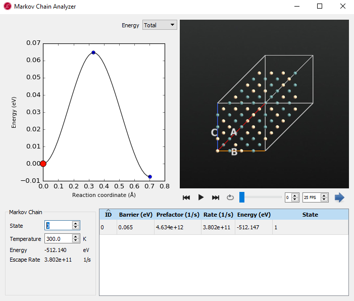
Select the  gID000 object in the
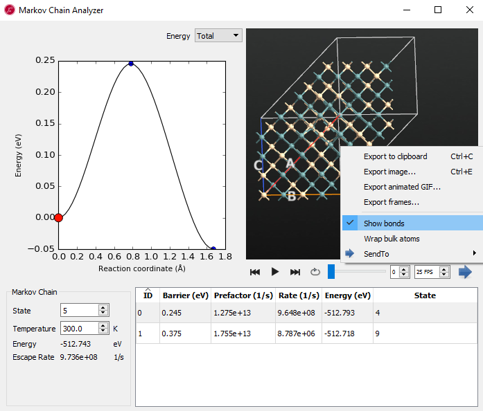
 akmc_markov_chain.hdf5 file on the Labfloor, and click the Markov Chain Analyzer in the right panel.
Examine the each state (here, state 0 and state 5 are shown in the below images) and use the play button  in the movie tool to see the diffusion and movement of atoms. From state 0, the system has a very low energy barrier of 0.065 eV towards state 1. When you look at the movie, it seems to be a kind of relaxation and not real diffusion.
State 0
From state 5 we have found saddle points that are connected to state 4 and state 9. They have relatively higher barriers than the one leading from state 0. When you see the movie, silicon and germanium are diffusing and exchanged in the vacancy. If you click the right mouse button on the structure window, you can show the bonds. It can be helpful to show the movement of the atoms when going along the energy diagram.
State 5
Note
Remember that you will probably have other results from a randomly generated alloy.
The Kinetic Monte Carlo object stores the time and state-to-state trajectory and is also able to take steps along the Markov chain (i.e. KMC steps). Select both objects,  in the
 akmc_kmc.hdf5 and in the akmc_markov_chain.hdf5, pressing the ctrl key, then see the activated Kinetic Monte Carlo Analyzer… in the right panel. The output should look like, but probably not be identical to, the one seen below:
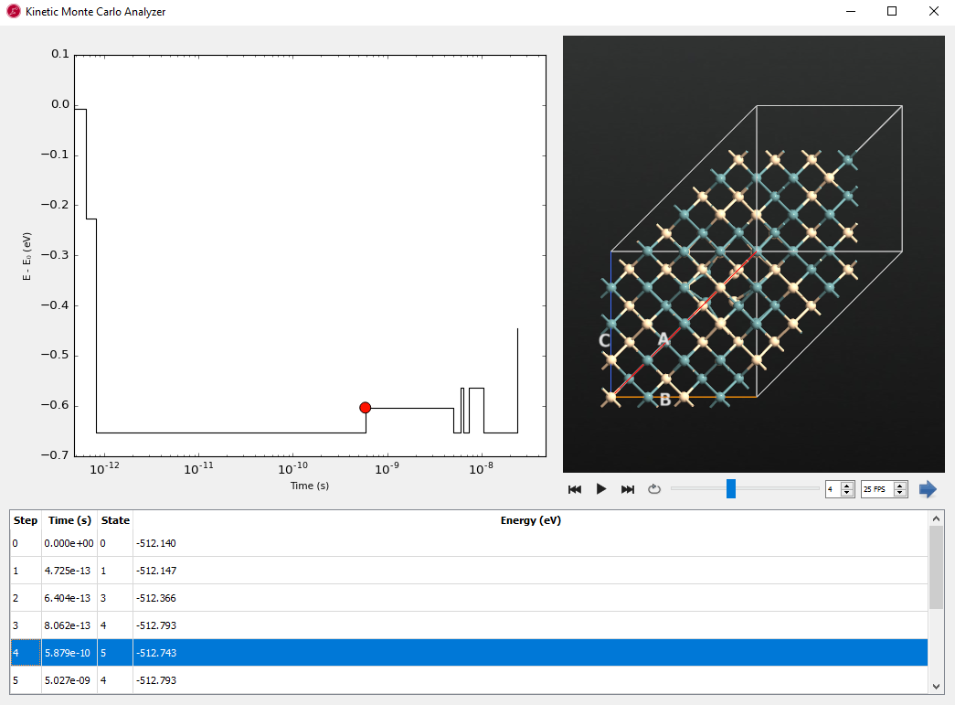
This analyzer shows the state-to-state trajectory along time from the Kinetic Monte Carlo simulation.
The KMC step, elapsed time, visited state id and energy are shown in the table. Click the movie button. You see the state to state dynamics with the energy vs. time plot. Since the plot is logarithmic on the time axis, the 0 and 1 steps near zero seconds cannot be seen clearly. You can find the different saddle states and staying time or escape time from each state. Starting from the initial state (0 eV), this plot shows the energy difference for other searched saddle points along the time.
In the LabFloor, click on the object in the akmc_kmc.hdf5 and select Text Representation from the panel on the right.
	# Item:  0
	# File:  C:\tutorial\akmc\akmc_kmc.nc
	# Title: akmc_kmc.nc - gID000
	# Type:  KineticMonteCarlo
    	Step #   Time (seconds)  State
        	0   0.00000000e+00      0
         	1   4.72548280e-13      1
         	2   6.40378862e-13      3
         	3   8.06232998e-13      4
         	4   5.87851546e-10      5
         	5   5.02734297e-09      4
         	6   5.98297032e-09      7
         	7   6.50322348e-09      4
         	8   7.34741500e-09      7
         	9   1.04551543e-08      4
        	10   2.38590351e-08      8
        	.
        	.
        	.
     		1501   9.97728735e-07      3
     		1502   9.99898062e-07      4
     		1503   1.00003149e-06      3
     		1504   1.00593170e-06      4
     		1505   1.00605679e-06      3
It includes the same information which we have seen in the Kinetic Monte Carlo Analyzer table. Here we show the results from a much longer simulation, with 500 saddle searches. The first column is the step number for the KMC algorithm, the second column represents the total elapsed time in the KMC simulation and the third column shows the current state number, which corresponds to a particular minimum energy configuration in the MarkovChain object. Note the break and how the time crosses 1 microsecond in the bottom text part ( step # 1501~1505 ), which is actually from the middle of the file: akmc_kmc_500.hdf5
Note
Do not confuse the KMC step and saddle point number. The saddle points are discovered as they represent the most likely events to be chosen in the KMC simulation. To ensure the accuracy of the simulation, each state in the Markov chain has an associated confidence. This confidence is an estimate of the probability that for each KMC step taken from that state, the correct event was chosen. Saddle searches are executed in each state until a user defined confidence level is reached. Once the confidence level is reached, the KMC simulation will proceed until a state is reached where the confidence is less than the target level.
The output above includes more KMC steps than the 500 saddle searches that was specified in the script. This shows that the KMC algorithm, to some degree, has been jumping back and forth between the same states. However, as AKMC is a stochastic method it is also entirely possible to see the opposite, with the total number of KMC steps being much smaller than the specified number of saddle searches. This behavior is also very system-dependent.
Note
Note how the final time is greater than a microsecond. This is a much longer timescale than we could probe using MD alone.
On the LabFloor you will also find an  akmc_log object. Open it by clicking on Text Representation. You should see a message equivalent to what is shown below. This shows the results of the 100 saddle searches you specified in the script.
# Item:  0
# File:  C:\tutorial\akmc\akmc_log.nc
# Title: akmc_log.nc - gID000
# Type:  AKMCLog
state id search number confidence  message
       0             0   0.000000  Found new state
       0             1   0.864665  Found saddle connecting to state 1 again
       0             2   0.950213  Found saddle connecting to state 1 again
       0             3   0.981684  Found saddle connecting to state 1 again
       0             4   0.993262  Found saddle connecting to state 1 again
       1             5   0.000000  Found new state
       1             6   0.000000  Found new state
       1             7   0.000000  No barrier was found between the end points of the NEB calculation. Check to see if there are enough images and that the NEB is converged.
       1             8   0.375441  Found saddle connecting to state 3 again
       1             9   0.375441  No barrier was found between the end points of the NEB calculation. Check to see if there are enough images and that the NEB is converged.
       1            10   0.375441  No barrier was found between the end points of the NEB calculation. Check to see if there are enough images and that the NEB is converged.
       1            11   0.840168  Found saddle connecting to state 2 again
       1            12   0.840168  No barrier was found between the end points of the NEB calculation. Check to see if there are enough images and that the NEB is converged.
       1            13   0.877314  Found saddle connecting to state 3 again
       1            14   0.923293  Found saddle connecting to state 2 again
       1            15   0.923293  No barrier was found between the end points of the NEB calculation. Check to see if there are enough images and that the NEB is converged.
       1            16   0.940208  Found saddle connecting to state 2 again
       1            17   0.940208  No barrier was found between the end points of the NEB calculation. Check to see if there are enough images and that the NEB is converged.
The first column is the id of the initial state used for the saddle search, the second column is the search number (out of the 100 saddle searches), the third column is the calculated confidence that the processes starting in the current basin are adequately sampled and the last column is the result of the search. In this case, the algorithm finds 1 new state and meets the confidence of 99% after 5 saddle searches starting from state 0, then go to state 1 (id 1). It finds a total number of 2 new states (states 2 and 3), 17 searches find a duplicate state and 6 searches find no new states for various reasons. The initial state from id 0 to id 1 has changed, showing that the KMC algorithm has taken a step to a new state, and the saddle searches then continue from there.
Conclusion
In this tutorial we examined how to perform an AKMC simulation for the diffusion in an alloy with a vacancy at 300K. The AKMC method is useful to search for saddle points near the initial state which are relevant on a microseconds time scale. When you run a longer simulation or search more saddle points, you can model timescales which are comparable to experiments aiming to understand the state-to-state dynamics.
In a real study it is always important to verify the results of a classical potential and re-optimizing the NEB’s describing the barriers using DFT, would be a good idea to determine pathways in the system more exactly.