Virtual Crystal Approximation for InGaAs random alloy simulations
Version: 2017
In this tutorial you will learn how to use the virtual crystal approximation (VCA) in order to simulate properties of random alloys with InxGa1-xAs as the specific system of interest. You will use VCA with the PBEsol exchange-correlation (xc) functional for determination of the lattice constant as a function of the In fraction \(x\), and then use VCA with the TB09-MGGA xc-functional to compute the band structures.
Introduction
Random alloys are becoming technologically important materials. SiGe is one of the best known materials for thermoelectric elements and InxGa1-xAs is a prime candidate to substitute or complement silicon in future CMOS devices. Simulations of both thermoelectric elements as well as transistor devices often refers to band structure parameters such as band gaps and effective masses. In a random alloy, one can calculate the so-called EffectiveBandstructure (EBS), which includes effects of the random disorder. However, EBS calculations require large unit cells and are rather time consuming. For more details, see the tutorial: Effective band structure of random alloy InGaAs.
A different approach to modeling a random alloy is to use the virtual crystal approximation (VCA), which is the topic of the present tutorial. In a VCA simulation of, for instance, InxGa1-xAs one creates a new, virtual atom, which is a mixture of In and Ga with appropriate weights. The actual calculation of e.g. lattice constants or band structures can then be performed on a primitive cell with only two atoms: the normal As atom and the virtual In-Ga atom. See also the manual page: VirtualCrystalBasisSet.
Compared with EBS calculations, VCA simulations are much less computationally demanding, since there is no requirement for large super cells. Conversely, VCA simulations do not capture any effects of disorder, as in the EBS approach. However, as it is shown in the EBS tutorial, the random disorder has a small effect on the band structure around the \(\Gamma\)-point, which is also the most important region for InGaAs. For this reason it makes good sense to study the band structure with VCA.
Setting up the VCA calculations for InxGa1-xAs
In the first part of the tutorial, you will calculate the lattice constant of InxGa1-xAs vs. In fraction x. You will be using the the GGA-type PBEsol exchange-correlation functional.
Open the Builder
 and add an InAs bulk configuration:
Send the InAs structure to the Script Generator.
In the Script Generator  go through the following points:
Add a New Calculator
 , open it and apply the settings:
Calculators: ATK-DFT:LCAO (default)
k-point sampling: 9x9x9.
Exchange correlation: PBES
Basis set: Change Arsenic to High.
Add an OptimizeGeometry
 object and open it.
Un-check Constrain Lattice Vectors to also optimize the lattice parameter.
Note
Note that we use Medium basis sets for all elements. It was changed to High in the Script Generator to make sure the basis set was printed in the script, allowing us to easily modify it.
Add a Bandstructure
 object and open it.
Set Points pr. segment to 100
Change the Brillouin zone route to L, G, X to just include a region around the \(\Gamma\)-point.
Note the filename - you will need it later.
Note
The particular choice of filename is not important, as we will change it later. In this way it is easy to do an automatic search and replace without changing other things by accident.
In order to use the VCA basis set, you need to modify the python script. Send the script to the Editor and find the lines:
basis_set = [
    BasisGGASG15.Arsenic_High,
    BasisGGASG15.Indium_Medium,
    ]
and replace them with the following lines:
VirtualCrystalBasis = VirtualCrystalBasisSet([BasisGGASG15.Indium_Medium,BasisGGASG15.Gallium_Medium], x=x)
basis_set = [
    VirtualCrystalBasis,
    BasisGGASG15.Arsenic_Medium,
    ]
In the first line the VirtualCrystalBasis is defined, based on regular basis sets of the SG15-Medium type. The VirtualCrystalBasis is constructed with:
A list of two basis sets.
A number \(0≤x≤1\), defining the fraction of the first basis set.
The VirtualCrystalBasis will be associated with atoms in the configuration corresponding to the first element in the list - in this case Indium. So we now have a configuration containing regular Arsenic, and an atom which is a tunable mix of In and Ga, represented by the In atom in the actual BulkConfiguration.
You can now calculate the lattice constant and band structure for InxGa1-xAs with an arbitrary value of \(x\). However, an advantage of VCA is the very short calculation time, so we would rather do calculations for many values of \(x\) to show the detailed dependence on \(x\). We therefore need to modify the script to loop over \(x\). Add the following lines at the top of the script:
# -*- coding: utf-8 -*-

x_range = numpy.linspace(0, 1.0, 11)
print('x_range', x_range)
for x in x_range:
    filename = 'ingaas-x%i.hdf5' % (x*100)
This will make a loop over \(x\) in intervals of 0.1, and create a separate file for each. Now go through the script (manually or with automatic replacement) and replace all instances of the filename (default is 'InAs.hdf5') with simply filename and indent all the lines as required by Python in a loop. Finally, we need to add the TB09-MGGA calculator, to get the band gap calculated with TB09-MGGA instead of PBES. Insert these lines between the OptimizeGeometry and Bandstructure parts, and make sure they have the correct indentation
    exchange_correlation = MGGA.TB09LDA

    calculator = LCAOCalculator(
        exchange_correlation=exchange_correlation,
        basis_set=basis_set,
        numerical_accuracy_parameters=numerical_accuracy_parameters,
        )

    bulk_configuration.setCalculator(calculator)
    bulk_configuration.update()
    nlsave(filename, bulk_configuration)
Read the script and make sure you understand what is being done and then run the calculation. It should take a couple of hours depending on hardware. Your script should look like this: vca-ingaas-full.py.
Note
For scientific use you should always carefully investigate if your numerical settings are converged. This includes in particular:
k-point sampling
Density mesh cutoff.
Choice of basis sets/pseudopotentials - and their influence on the required mesh cutoff.
Analyzing the results for VCA with InxGa1-xAs
Lattice constants
When the calculations are done, the results can be visualized with the plot-lattice-constant.py script. The lattice constant is plotted vs. the In fraction \(x\).
The solid line is an analytical expression which is based on experimental room temperature lattice constants [1], while the computed results correspond to zero temperature. Experimental low temperature lattice constants for GaAs (\(x=0\)) and InAs (\(x=1\)) lie slightly below the solid line [2].
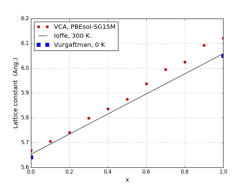
We see that the experimental lattice constants are well reproduced in the Ga-rich region on the left of the figure, while the deviation is higher, about 1 %, in the In-rich region on the right. This is in line with general expectations, as PBEsol is designed to give accurate lattice constants, while GGA-type functionals generally overestimate them.
Band gaps - self-consistent TB09-MGGA
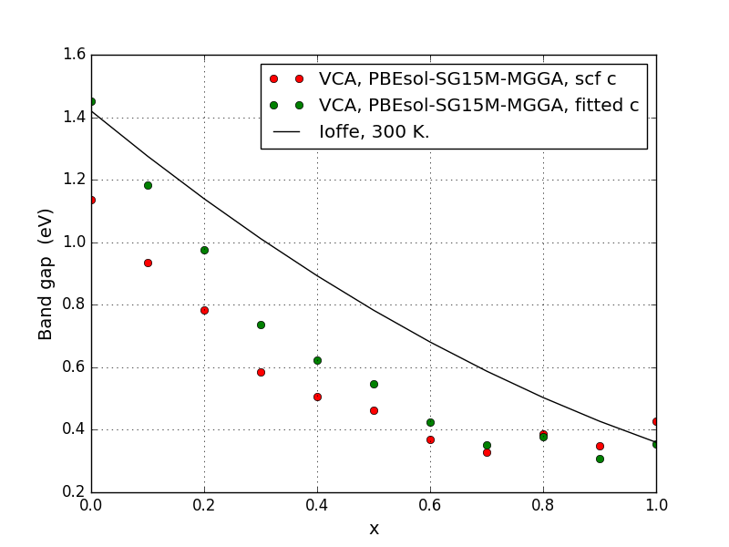
We also calculated bandstructures, from which we can extract the band gaps with the following script: plot-band-gaps.py. This will produce this plot:

We see that the band gaps show a qualitatively correct trend, but with rather large deviations in the Ga-rich region on the left and a bit of an oscillation on the right. Fortunately, it is possible to fit the c-parameter of TB09-MGGA to reproduce the correct band gaps of the end-points, which should also improve the band gaps in the intermediate region.
Band gaps - TB09-MGGA with fitted c-parameter
In order to fit the c-parameter, we need to re-visit the calculations for \(x=0\) and \(x=1\). The procedure for doing the fitting is rather straightforward and described in this tutorial: Meta-GGA and 2D confined InAs.
For our combination of computational parameters, we find that a c-parameter of 1.1331 optimizes the band gap of InAs and a c-parameter of 1.2680 optimizes the band gap of GaAs. We cannot know beforehand which parameter values optimize the band gap for the various compositions in between, so the most straightforward choice, is to simply make a linear interpolation between the two values.
We make a modified version of the previous script, which reads in the finished calculations, re-calculates with TB09-MGGA with a linear interpolation between the fitted c-parameter values and computes and saves a bandstructure:
# -*- coding: utf-8 -*-
x_range = numpy.linspace(0, 1.0, 11)
print('x_range', x_range)
for x in x_range:
    filename = 'ingaas-x%i.hdf5' % (x*100)

    bulk_configuration=nlread(filename,BulkConfiguration)[-1]
    old_calculator=bulk_configuration.calculator()

    # Interpolated fitted c
    c = 1.2679609982 - 0.13488609 * x
    exchange_correlation = MGGA.TB09LDA(c=c)

    calculator = old_calculator(
        exchange_correlation=exchange_correlation,
        )

    bulk_configuration.setCalculator(calculator)
    bulk_configuration.update()

    bandstructure = Bandstructure(
        configuration=bulk_configuration,
        route=['L', 'G', 'X'],
        points_per_segment=200,
        bands_above_fermi_level=All
        )
    nlsave(filename, bandstructure)
Run the script in the same folder, to re-do the TB09-MGGA calculations with a fitted c-parameter and get the corresponding bandstructures. We also modify the plotting script to include both datasets (plot-both-band-gaps.py), giving us this plot:
We see that this has improved the band gaps quite a bit in the Ga-rich part on the left, while the improvement is smaller in the In-rich part on the right.
Calculating effective masses
It is also possible to calculate the effective mass of the electrons as a function of \(x\). See this tutorial: Effective mass of electrons in silicon, for general information on calculation of effective masses. The script is equivalent to the one used for the new TB09-MGGA calculations, and also plots the data, and can be found here: effective-masses.py. It will give this plot:

We see that the effective mass of GaAs is overestimated, leading to an overall distortion of the shape of the curve. However, it does capture the overall downwards trend in the effective mass from GaAs to InAs.
Summary and discussion
You have now learned how to use the VCA in order to calculate structural properties (lattice constants) and band structure properties (band gaps and effective masses) of InxGa1-xAs. The lattice constants were well-reproduced, and while the fundamental band gap at the \(\Gamma\) point came out satisfyingly with the fitted TB09-MGGA c-parameter, the effective masses were not as accurate.
When using the VCA you must be aware that you are ignoring all effects of the random disorder. You are implicitly assuming that Bloch’s theorem applies and that the band structure is a well-defined quantity (or, alternatively that k is a good quantum number). This might, however, not always be the case, as shown in the calculations in the tutorial Effective band structure of random alloy InGaAs, which includes the random disorder. However, the effective band structure calculations also indicate that close to the \(\Gamma\) point, the band structure is indeed well-defined in InxGa1-xAs. In that case it makes good sense to study the band structure details (effective mass, band gap, strain dependence, etc.) with the VCA, which is computationally much easier than the effective band structure calculation, which requires large supercells.