Generating Amorphous Structures
Introduction
Amorphous solid materials become more and more important for a broad spectrum of technologies. In contrast to crystal structures, which are usually well- defined, it is, however, rather difficult to obtain the amorphous structure of a given material in order to perform atomistic simulations. This tutorial gives you some guidelines about generating amorphous structures in QuantumATK using molecular dynamics (MD) simulations at different levels of precision.
Amorphous structures, i.e. structures without any periodic order of the building atoms or molecules, can be found in various kinds of materials, e.g. glass or polymers. Their mechanical and electronic properties often differ quite substantially from the respective crystal. For example, the thermal expansion coefficient of amorphous silica is about one order of magnitude lower than the corresponding value for quartz-crystals.
Consequently, there is a growing interest in the employment in amorphous materials, to tailor various material and device properties in a desired way. In this effort, atomistic simulations can help to understand the behaviour of amorphous strucures at the nano- and microscale.
It is, however, not always straightforward to obtain a suitable amorphous structure of a given material for such simulations. In contrast to the corresponding crystal structure there is no unique unit cell or supercell representation, as the structure inherently bears large degree of randomness. Instead, one should ideally consider an ensemble of realizations of such structures, which is in reality often prohibited by the computational cost of the required calculations.
In this tutorial, you will learn how you can generate amorphous structures that can serve as representative examples and input configurations for further simulations, based on DFT or classical force field methods.
You will learn how to use classical force field MD simulations to obtain a first starting structure of the amorphous material, which can in a second step be refined using semi-empirical or DFT molecular dynamics, when the focus is set on electronic properties.
As there is in general no universally valid recipe to create amorphous structures, the most suitable protocol for a given material depends on a lot of factors, such as the availability of a reliable empirical potential, the desired size of the supercell, the disposable computational resources, etc. This tutorial will therefore only provide a guideline, rather than a rigid protocol, to generate amorphous structures, which might have to be modified according to the particular application at hand.
You will simulate amorphous silicon dioxide, often referred to as fused silica or fused quartz, which is one of the most widely used amorphous materials, e.g. in conventional or specialized glass and also in the semiconductor industry.
You will also learn how to create interface structures between crystal and amorphous regions.
If you don’t have much experience in MD simulations, you can start with the How to Setup Basic Molecular Dynamics Simulations, which will help you to become familiar with the MD functionality in QuantumATK.
Note
The simulations in this tutorial use a comparably small number of steps to demonstrate within a reasonable time the principle of generating amorphous structures. For actual production simulations, in order to achieve more reliable amorphous samples with a low amount of structural defects, you should use much longer simulation times. Typically, a melt-quench cycle comprises at least several hundred picoseconds, or even several nanoseconds. Take a look at the references of this tutorial to get an overview over common simulation protocols.
Amorphous Structure Generation with Classical MD Simulations
The most common way to generate amorphous structures is to mimic the experimental protocol of melting a crystal and cooling it down again by using MD simulations [1], [2]. Although cooling rates accessible in MD simulations can not be chosen as low as the experimental cooling rates, this procedure gives satisfactory results in many cases. The quality of the resulting amorphous structures of course depends much on the ability of the employed force field to describe the material, also further away from equilibrium conditions.
Setting up the Geometry
You will start from a crystalline SiO2 system, specifically a cristobalite structure. In contrast to e.g. quartz, the cristobalite unit cell can easily be transformed into an orthogonal cell, which makes the simulation much more convenient. Moreover, the density of cristobalite is very similar to the experimental density of amorphous silica, being 2.2 g/cm3.
Open the Builder and click and search
for “sio2”. Select the cristobalite structure and add it to the Stash. To
transform it into an orthogonal cell, click on
on the right-hand-side panel. Click Conventional and then
Transform. For cristobalite this will create a cubic supercell.
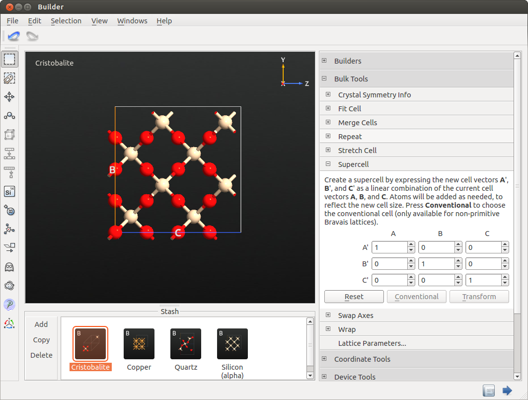
The resulting cell is too small yet to be a useful container for an amorphous structure, as the periodic boundary conditions would still enforce a certain amount of crystallinity. Therefore, repeat the cell by opening , and apply a 3 x 3 x 3 repetition. This cell, containing 648 atoms, will be the starting structure for the MD simulations.
Setting up the Simulation
Send the configuration to the ScriptGenerator. Add a and an block to the script panel.
Double-click on the NewCalculator block and select the ATK-ForceField
calculator with the Pedone_Fe2_2006 potential [3]. Uncheck Print and
Save. Close the NewCalculator widget by clicking Ok.
Note
For QuantumATK-versions older than 2017, the ATK-ForceField calculator can be found under the name ATK-Classical.
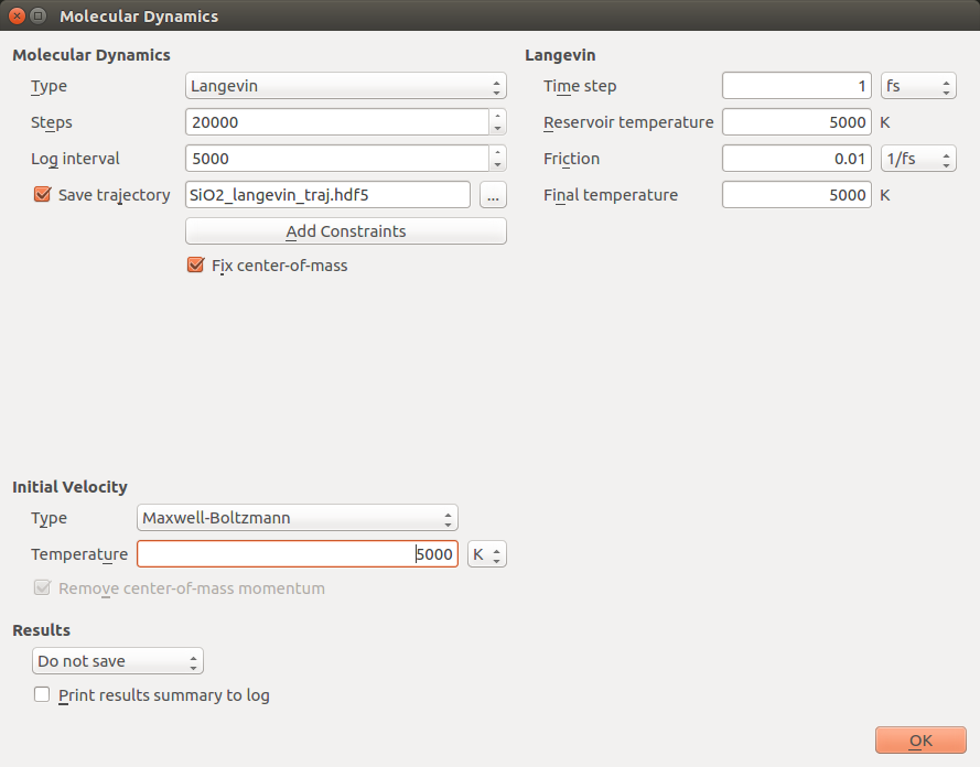
Now double-click on the MolecularDynamics block. To melt the crystal, you
will start with simulations at a very high temperature of 5000 K. As the
primary purpose of this initial simulation is to randomize the arrangement of
the atoms, no pressure coupling is needed at this stage. Therefore you should
select a Type, which gives you an NVT ensemble (take a look at the
How to Setup Basic Molecular Dynamics Simulations for a more detailed documentation of MD simulation
types in ATK). A good choice is the Langevin thermostat, as it produces
a very tight coupling to the heat bath and therefore prevents single atoms
from becoming too hot and possibly destabilizing the system.
Set the Steps to 20 000, the Log interval to 5000, and the filename to
save the trajectory to SiO2_5000K_langevin_traj.hdf5. In the
Initial Velocity group box, select the Maxwell-Boltzmann type at a
temperature of 5000 K.
Enter the same temperature value of 5000 K in the Langevin group box in
the Reservoir temperature field. Leave the remaining settings at their
default values. Finally, select Do not Save under Results (as the
trajectory is already being saved).
Use the  button to send the script to the Editor in order to
make some additional changes.
button to send the script to the Editor in order to
make some additional changes.
Facilitating the Melting Process via Lowering the Density
In some cases, particularly when you attempt to melt comparably small supercells, you may sometimes observe that the crystal does not melt even at temperatures far beyond the experimental melting point. A possible reason for this behavior, apart from deficiencies of the employed classical potential, is that crystal structures are additionally stabilized by the periodic boundary conditions, and, generally, artifacts of the periodic boundary increases with decreasing size of the supercell. Another aspect that has to be kept in mind is that the fixed volume of the cell is likely to produce a large system pressure at high temperatures, which can additionally elevate the melting point temperature or in some cases thermodynamically favor another crystal phase over the liquid phase.
Note
If you don’t expect or experience any problems with melting the structure, you can run the script as is, and skip the rest of this section.
To facilitate melting, you can slightly increase the cell volume to artificially lower the density. In the script this is achieved by multiplying the the lengths of the cell vectors by a factor of e.g. 1.1.
Modify the block in which the lattice is defined, as shown in the following script:
# Set up lattice
# Define a scale factor
scale_cell = 1.1
# Scale all 3 cell vectors by this factor
vector_a = [21.498*scale_cell, 0.0, 0.0]*Angstrom
vector_b = [0.0, 21.498*scale_cell, 0.0]*Angstrom
vector_c = [0.0, 0.0, 21.498*scale_cell]*Angstrom
lattice = UnitCell(vector_a, vector_b, vector_c)
The exact value of the scaling factor does not play a crucial role, and can be increased as long as you still detect some residual crystallinity after annealing the system at 5000 K.
Send the modified script to the Job Manager and run the simulation.
It will take a couple of minutes to complete the simulation. If you select the
produced trajectory file on the LabFloor and visualize it with the
Movie Tool, you will see the atoms moving around in a chaotic fashion, as
they frequently cross the periodic boundaries of the cell. To take a better
look at the structure, send the last snapshot of the movie to the Builder via
the button in the lower right-hand corner of the Movie Tool.
In the Builder you can fold all atoms that have crossed the periodic boundaries back into the simulation cell by clicking .
The final structure may look similar to the example below.
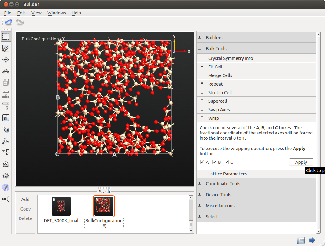
Due to the artificially decreased density the atoms cluster in certain regions, producing an inhomogeneous distribution. However, the purpose of the procedure, i.e. a complete randomization of the previously crystalline structure has been fulfilled very well.
To recover the original density, send this configuration to the ScriptGenerator and repeat exactly the same steps described above (i.e. prepare a script containing a NewCalculator and a MolecularDynamics block with the described settings and send it to the Editor), but now divide the cell vectors by the same scaling factor 1.1 (respectively the factor you have used to lower the density) instead of multiplying them. This procedure will compress the system and recover the original density of the cristobalite structure. Run this simulation at 5000 K for 20 000 steps to equilibrate the silica melt at the new density, send the final configuration from the Movie Tool to the Builder, and the configuration.
Cooling the Structure and Adjusting the Density
If you inspect the resulting structure with respect to the local atomic arrangements, you will encounter many structural defects, such as undercoordinated atoms (e.g. oxygen atoms with only one silicon neighbor).
This is because the resulting amorphous system represents a snapshot of the material in the liquid state at very high temperature. The ultimate goal is usually the generation of solid amorphous material, i.e. at temperatures well below the glass-transition temperature Tg. Therefore, you will perform a MD simulation where the temperature decreases linearly at each time step to cool the system to the desired temperature.
Although real amorphous structures always contain a certain amount of structural defects, the goal of such a cooling simulation is to perform the temperature change as slowly as possible to allow the system to reduce the number of defects as much as possible [2]. Unfortunately, the limited accessible simulation time often requires the use of very high cooling rates compared to experimental settings. The parameters, suggested in the following paragraphs, have been chosen to allow for a rather quick demonstration of the principle of the structure generation, which may not be the optimal choice for production simulations. To obtain a more reliable amorphous structure, consider increasing the simulation time, which will decrease the cooling rate.
Another important parameter is the density of the amorphous structure. There are essentially two different possibilities for how to deal with this matter.
One way is to adjust the system volume a priori, to obtain the desired experimental amorphous density and leave the volume at this fixed density throughout the cooling simulation [1]. This technique is the preferred method when the accessible simulation time is very limited, e.g. in DFT-MD simulations. However, it can lead to large residual stress values in the final systems.
The alternative way is to adjust the density continuously during the cooling simulation by coupling the system volume to a barostat at ambient pressure [2]. Here, the resulting density will depend on the quality of the employed potential and you should check whether it is consistent with experimental values and, in case of large deviations, consider repeating the simulations at fixed volume.
In this example you will use the second technique, i.e. use a barostat to control the system pressure.
Prepare the cooling simulation by sending the last snapshot of the previous
simulation to the Builder via the button. Fold the
coordinates back into the simulation cell by using the
tool, as described above. Send the configuration to the ScriptGenerator.
Add a and an block. In the NewCalculator widget, use the same
settings as in the previous simulations.
Open the MolecularDynamics settings. Select the NPT Martyna Tobias Klein type.
Select 50 000 steps, a log interval of 1000, and set the trajectory name to
SiO2_NPT_cool_to_300K.hdf5. Select Maxwell-Boltzmann initial velocities
corresponding to 5000 K.
Change the Reservoir temperature to 5000 K. To cool the system down to
room temperature you need to change the Final temperature to 300 K. This
will result in a linear decrease of the current reservoir temperature from
5000 K to 300 K during the MD simulation.
Leave the remaining parameters at their default values.

Send the simulation workflow to the Job Manager and execute it. It will take some time to complete.
The simulations should run without problems for this system. However, if you encounter extreme, non-stationary cell size fluctuations, or the formation of pronounced vacuum pores during the NPT runs at high temperatures, you can consider switching on the barostat coupling after reaching lower temperatures, e.g. roughly in the region of the suspected glass temperature. You could, for example, use the NVT Nose Hoover thermostat to cool the system from 5000 K to 2000 K at constant volume, and the NPT Martyna Tobias Klein barostat to cool it from 2000 K to 300 K.
Analyzing the Structure
After the simulations have finished, you can take a look at the trajectories using the Movie Tool or the Viewer.

If you have a close look at the local atomic arrangements, you will notice that almost the entire structure is composed of slightly distorted, vertex- sharing tetrahedra formed by SiO4 units. Additionally, you may encounter some few coordination faults.
For a quantitative assessment, select the SiO2_300K_NPT_traj.hdf5 file
on the Lab Floor and open it with the MD Analyzer tool. Here, you can
perform various kinds of analyses of the MD trajectory. For amorphous systems,
we are particularly interested in the radial distribution function (RDF). To
perform such an analysis, increase the cutoff radius r:sub:max to 8.0 Å,
select Silicon as Element 1, select Oxygen as Element 2, and
click Plot to display the RDF between these two elements. To discard the
high temperature part of the trajectory, you can set the t:sub:min parameter
to 40 ps to analyze only the last 10 ps of the trajectory.
Instead of sharp single lines, as in a crystal structure, you will find a distribution of broadened peaks, which is characteristic for an amorphous structure. You can plot the RDF for different element pairs or between all elements.
The number of structural defects can be investigated by selecting the
Coordination number analysis. Select, for example Silicon and Oxygen as
Element 1, respectively Element 2, to calculate the coordination of
silicon with oxygen atoms. Set the cutoff radius to 2.5 Å, according to the
first minima in the RDF curve. Click Plot to create the distribution of
coordination numbers. You will see that most of the silicon atoms
have a coordination number of four, and only a tiny fraction
have a lower coordination. Now switch the elements to calculate the
coordination number of the oxygen atoms. Click Plot to add the
distribution to the existing plot. Again, the majority of oxygen atoms
exhibit its regular coordination number of two, whereas only few atoms are
undercoordinated. Switch the Analysis Type to Time Evolution to plot
how the number of atoms with a given coordination number changes during the
cooling simulation. The following example shows that the number of one-fold
coordinated oxygen atoms decreases during the simulation, while the number of
two-fold coordinated atoms increase. This reduction of coordination defects
could possibly be enhanced further by choosing a slower cooling rate (i.e.
longer simulation time).

The MD Analyzer provides a large number of different analysis quantities that can be invoked with a few clicks. Feel free to explore its functions. For example, take a look at the Angular distribution function for Silicon-Oxygen-Silicon angles, or at the Neutron scattering function.
The density of the generated amorphous silica cell can be calculated from the volume of the cell, which can be found in the Builder under , and the numbers of the elements and their respective masses. For the present example, you should obtain a value around 2.6 g/cm3. This value is a little higher than the experimental value of 2.2 g/cm3, which must be considered a small shortcoming of the potential. To obtain exactly the experimental value, you may repeat the cooling simulation with a fixed volume, adjusted to reproduce the desired density. The NVT Nose-Hoover thermostat with a linear decrease in temperature might be the right method for such simulations.
The final result can be used as an input configuration for subsequent static calculations or MD simulations to calculate additional properties of interest. However, you should keep in mind that the generated configuration represents only one possible snapshot out of the amorphous ensemble. This means that in order to obtain meaningful results, you should average over several different samples.
Refining Amorphous Structures
You can refine the structure obtained via classical MD to compensate some of the possible shortcomings of the force field. This becomes particularly beneficial if you intend to calculate additional properties of the amorphous material based on semi-empirical or quantum mechanical calculations, e.g. tight-binding (TB) or density-functional-theory (DFT).
The fastest and easiest way is to perform only a TB or DFT geometry optimization to bring the configuration to the nearest energy minimum. This will primarily improve locally distorted geometries, but is not expected to fix connectivity defects.
A more profound refinement can be achieved by a short TB/DFT MD annealing and cooling procedure [1]. As these simulation are quite time-consuming they are suited predominantly for smaller systems comprising around 100-200 atoms.
In the following you will be guided through a brief example considering a small silica system with the ATK-DFT calculator. Since the accessible time in DFT-MD simulations is very limited, which makes a reliable constant pressure equilibration difficult and computationally expensive, you will perform the classical and DFT-MD simulations in this particular example at constant volume. The density will remain at the value of the cristobalite crystal, which is very close to the experimental density of amorphous silica.
Setting up the classical simulation
Before running the DFT simulation, you first have to prepare an amorphous cell using a classical MD simulation. These steps essentially follow the protocol outlined in the previous section.
Prepare a cristobalite cell in the same way as described in the previous section, but use only 2x2x1 repetitions in the tool of the Builder. This will create a cell containing 96 atoms. Due to this repetition the cell the box size is 14.33 x 14.33 x 7.17 Å3, i.e. the z-direction is thinner compared to the other directions, which might introduce an increased ordering in this direction. To avoid such effects, we will transform the cell to a cubic shape, which has the same volume as the original cell. The final cell size shall therefore be 11.375 x 11.375 x 11.375 Å3. You will perform this shape transformation in two steps during the high temperature simulations where the system is in a liquid state.
The first step comprises setting up a simulation, in exactly the same way as described above, i.e., adding the ATK-ForceField calculator with the Pedone_Fe3_2006 potential and a MolecularDyncamics block with the Langevin type, a step number of 20 000, and a temperature of 5000 K. Send the resulting script to the Editor. To achieve a lower density and therefore facilitate the melting, increase the length of the C-vector of the box to its final value of 11.375 Å:
# Set up lattice
vector_a = [14.332, 0.0, 0.0]*Angstrom
vector_b = [0.0, 14.332, 0.0]*Angstrom
# Previous C-vector:
# vector_c = [0.0, 0.0, 7.166]*Angstrom
# New C-vector:
vector_c = [0.0, 0.0, 11.375]*Angstrom
lattice = UnitCell(vector_a, vector_b, vector_c)
Run the simulation and send the final snapshot from the Movie Tool to the Builder. Wrap the configuration, set up exactly the same simulation script as in the previous simulation, and send it again to the Editor.
The cell volume has to be reduced to restore the original cristobalite density. Instead of resetting the C-vector to the original value, you can now set the lengths of the A- and B-vectors to 11.375 Å, too, in order to obtain a cubic cell. Run the simulation.
Send the final snapshot to the ScriptGenerator, add the same ATK- Classical calculator as described above, and an block. In the MolecularDynamics settings, select the NVT Nose-Hoover type, which allows to use a linear decrease in temperature. Adjust the settings as shown in the following screenshot.
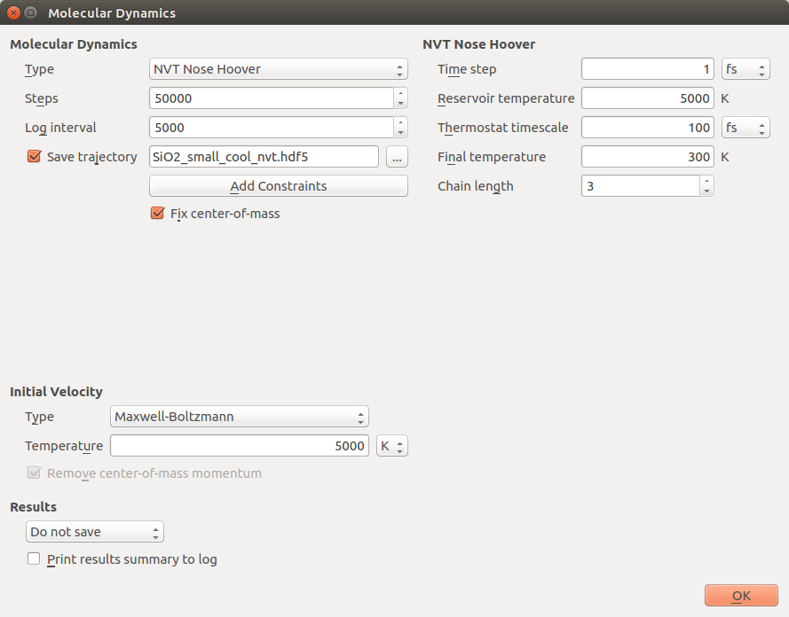
These thermostat settings will invoke a linear decrease of the reservoir temperature from 5000 K to 300 K over 50 picoseconds.
Run the simulation. Send the final snapshot via to the ScriptGenerator.
Setting up the DFT simulation
In the following you will perform an MD simulation using the ATK-DFT calculator in ATK to anneal the structure and cool it down to room temperature. MD simulations are rather expensive in terms of computational time. In order to generate amorphous structures, it is not absolutely crucial to obtain accurately converged energies. The suggested settings in the present example will therefore employ parameters, whose accuracy is slightly decreased with respect to the default values to accelerate the calculations. However, before you start the DFT simulations, be aware that these simulations can take very long time, up to several days, so it is recommended to run them on a cluster.
To set up the simulation script, add a and two
blocks. In the NewCalculator
settings select ATK-DFT calculator. Open the calculator widget to adjust
some of the settings. In the Iteration control parameters increase the
Tolerance to 0.001 Hartree. In the Basis set/exchange correlation
settings, change the exchange correlation Type to GGA. Next, change the
basis sets from DoubleZetaPolarized to SingleZetaPolarized.
Depending on your computational resources you may of course choose more accurate settings here, in particular when aiming at production simulations.
Close the NewCalculator settings by clicking Ok.
Add two blocks to the script.
Open the first block. Here, you will set up a short annealing simulation at
3000 K. Therefore, select the Langevin type, set the number of steps to 500
and the log interval to 20. Choose an appropriate trajectory filename, e.g.
traj-sio2-DFT-MD-3000K.hdf5, select Maxwell-Boltzmann initial
velocities at 3000 K and a reservoir temperature of 3000 K, as well. Finally,
uncheck Save and Print and close the settings.
Open the second MolecularDynamics block. In this simulation you will rapidly quench the system from 3000 K to 300 K. Use again the Langevin Type, set the number of steps to 1000 and the log interval to 20. Select again Maxwell-Boltzmann initial velocities at 3000 K. To cool the system during the simulation set the reservoir temperature to 300 K now, as if the system was transferred from a very hot reservoir to a heat bath at room temperature. Regarding the short simulation time this method is more efficient than using a linear decrease in the reservoir temperature via the NVT Nose-Hoover chain thermostat. Close the widget and run the simulation.
After the simulations have finished, the movie of the second phase, i.e. the quenching simulation, should look similar to the following.
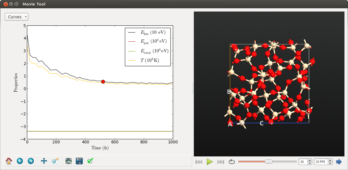
The temperature decays from the initial value of 3000 K to room temperature. Of course, this rapid quenching within 1 ps is only a rough approximation to the experimental procedure.
Depending on the properties one is interested in calculating, one can continue from the final configuration and perform a DFT geometry optimization.
Creating Crystal/Amorphous Interfaces
A particularly interesting application is given by interfaces between crystal and amorphous structures, as the local properties in proximity of the interface are largely unknown. Such systems can easily be created in the QuantumATK-Builder.
If the crystal is of the same material as the amorphous region, you can start by preparing the crystal configuration. The desired interface plane can be created using the tool in the Builder. Make a copy of the configuration. The latter system will serve as the basis to create the amorphous structure, as their surface areas already match exactly.
The following example considers the interface between quartz and amorphous silica. The initial structure is built in the tool by selecting the (10-10) surface and a 4x3 surface cell. Create a Periodic (bulk-like) supercell with a thickness of 12 layers. Perform a geometry optimization of the structure and the cell vectors, using again the ATK-ForceField Pedone_2006_Fe3 calculator, and save the final configuration to a HDF5 file. Drag and drop the file to the Builder, and use it as the initial structure for the amorphous cell.
Prepare the amorphous cell via the same simulation protocol as described
above, but apply the pressure coupling only to the Z-axis to preserve the
lateral cell dimensions. Unidirectional pressure coupling can be selected in
the MolecularDynamics settings, using NPT Martyna Tobias Klein. To couple the
barostat only to the Z-component, first uncheck Isotropic pressure and then uncheck all boxes in the Pressure coupling
group box, apart from the zz box.
After creating the amorphous supercell, you can join the optimized crystal and amorphous cell using the tool in the Builder panel. Therefore, you can simply drag and drop the configurations from the Stash to First and Second field in the . The builder should automatically detect suitable separations of both cells.
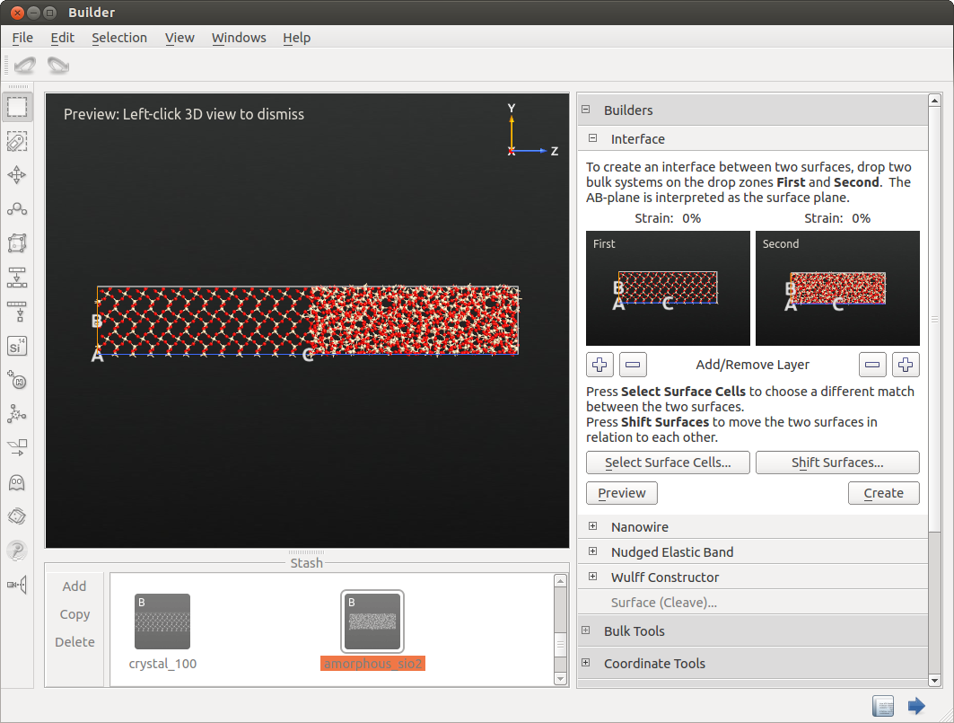
Click Create to finalize the build process and send the interface
configuration to the ScriptGenerator.
Tip
You can learn more about the Interface Builder in the Technical Notes on Interface Builder.
If you zoom into the interface, you will find many defects, such as dangling bonds. Most of these defects can often be healed by an annealing simulation using classical potentials, even if such potentials are not explicitly designed to include chemical reactions.
Add a , an , and an block. After selecting the desired calculator settings, in this case the Pedone_2006_Fe3-potential, open the OptimizeGeometry widget.
After the interface creation there will probably be many artificially
close atomic distances, which will cause a subsequent MD simulation to be
unstable. To remove these large forces from the interface, you will first run
a geometry optimization. The Force tolerance does not need to be
extremely low, so you can set a value of 0.5 eV/Å. Increase the Maximum
number of steps to 1000. Uncheck the Print box, rename the output file
to interface_optimized.hdf5, and close the OptimizeGeometry
settings.
Open the first MolecularDynamics settings. During the MD annealing you
should fix the atoms in the central crystal region to prevent the crystal
region from melting. To this aim, click on Add constraints to open the
Constraints Editor. In the presenter window, draw a rectangle around the
central atoms of the crystal region to select them, click Add tag from
selection, and select Fixed atoms constraints for this group in the
table on the side of the widget.

Close the Constraints Editor.
In the MolecularDynamics widget, select NVT Nose-Hoover Chain, set the number of steps to 50 000 and the log interval to 2000 steps. First, you should anneal your structure at a temperature high enough to allow for local rearrangements of atoms, thus facilitating the healing of interfacial coordination defects, but not too high, to prevent melting of the global structure. A temperature of 1500 K is suitable for this purpose. Enter this temperature into the initial velocity temperature and the reservoir temperature fields.
Now add another block to the
script for the cooling simulation. Double-click it and open the Constraints
Editor. The previously selected group “Selection 0” should already be
present in the table. Select Fixed atom constraints for this group and
close the widget. In the MolecularDynamics widget, select the NVT Nose-
Hoover Chain thermostat, 50 000 steps, a log interval of 2000 steps, and
Configuration velocities as initial velocities. In the thermostat settings
set a Reservoir temperature of 1500 K and a Final temperature of 300 K
to achieve a temperature decrease during the simulation.
Run the simulation by sending the script to the Job Manager.
To finalize the structure, you should run another NPT simulation, this time
without any constraints. Use the NPT Martyna Tobias Klein barostat and
uncheck Isotropic pressure as well as all stress coupling boxes except for
the zz-box to equilibrate only the cell height perpendicular to the
interface plane. Run the simulation for 50 000 steps at 300 K to obtain a room
temperature amorphous/crystal interface structure.
Further Examples
Finally, this section provides some further examples of generating amorphous structures of the technologically relevant materials alumina, titania, and hafnia.
Al2O3
For the creation of an amorphous alumina sample, you can essentially follow the protocol outlined in Refs. [3] and [4]. To use the same classical potential [5], you can either select Matsui_CaMgAlSiO_1994, or, if you use an older version of QuantumATK where this potential is not available, download the Python script attached to this tutorial. If you copy and paste its contents to the top of your simulation script, the potential will be available in the simulation.
To set up the system, you need to import the crystal structure of
\(\alpha\)-Al2O3 into the Builder. To this aim, download the
Al2O3_corundum_AMS_DATA.cif file. In the
Builder, click and open the file. For
a more convenient handling in MD simulations the trigonal cell should be
converted into an orthogonal cell. The are several ways to achieve this. One
possibility is to open the tool.
Select (10-10) Miller indices, click Next and select a 3x1 surface
lattice. Click Next and select a Periodic (bulk-like) cell with a
thickness of 4. Click Finish to obtain an orthogonal supercell containing
360 atoms.
Now, you should proceed similar to the protocol outlined above, with the exception that the density will be fixed to 3.175 g/cm3 (as proposed in Ref. [4]) during the cooling simulations. The entire protocol reads as follows:
Run a high temperature MD simulation at 5000 K and artificially reduced density.
Cool the system to 3000 K using the NVT Nose-Hoover thermostat.
Compress the system to the desired amorphous density.
Anneal at 3000 K.
Slowly cool the system to room temperature.
Run a final simulation at room temperature to calculate observables.
Send the orthogonal cell to the ScriptGenerator to set up a basic molecular dynamics script. Add a and two block.
In the NewCalculator block, select ATK-ForceField and the Matsui_CaMgAlSiO_1994 potential.
In the first MolecularDynamics block select the NVT Nose-Hoover
thermostat, 150 000 steps, a log interval of 5000 steps and uncheck the Save
trajectory box. Set the initial velocities to a Maxwell-Boltzmann-
distribution at 5000 K. Set the reservoir temperature to 5000 K and the final
temperature to 3000 K. The remaining parameters should be kept at the default
values. Finally, uncheck Save and Print, close the calculator widget,
and send the script to the Editor.
The second MolecularDynamics block should have similar settings, but 300 000 steps, a reservoir temperature of 3000 K and a final temperature of 300 K.
To obtain an artificially reduced density you should again multiply all three lattice vectors with 1.1, as explained above.
This first MolecularDynamics sequence yields a liquid system at 3000 K and
lowered density. Based on this system, the density should be adjusted to
achieve the target density of 3.175 g/cm3. As it is often cumbersome to
calculate the macroscopic density of an atomic cell and to obtain the exact
scaling factors for the cell vectors by hand, this can conveniently be
achieved using the QuantumATK unit engine by inserting the following piece of code in
the simulation script, right before the second MolecularDynamics block
(i.e. after the line bulk_configuration = md_trajectory.lastImage()):
# Get the volume and the lattice vectors of the cell.
V = bulk_configuration.bravaisLattice().unitCellVolume()
lattice_vectors = bulk_configuration.bravaisLattice().primitiveVectors()
# Get the coordinates and the elements.
fractional_coordinates = bulk_configuration.fractionalCoordinates()
elements = bulk_configuration.elements()
# The total and species-resolved number of atoms.
N = len(elements)
N_Al = len(numpy.where(numpy.array(elements)==Aluminum)[0])
N_O  = len(numpy.where(numpy.array(elements)==Oxygen)[0])
# Calculate the current density
density = (N_Al*Aluminium.atomicMass() + N_O*Oxygen.atomicMass())/V
# Get the density in g/cm**3
density = density.inUnitsOf(kiloGram/Meter**3)/1000.0
target_density = 3.175
# Calculate the scaling factor for the lattice vectors.
scale_factor = (density/target_density)**(1.0/3)
# Scale the lattice vectors.
lattice_vectors = lattice_vectors*scale_factor
# Define a new cell.
new_lattice = UnitCell(lattice_vectors[0], lattice_vectors[1], lattice_vectors[2])
# Set up configuration
bulk_configuration = BulkConfiguration(
    bravais_lattice=new_lattice,
    elements=elements,
    fractional_coordinates=fractional_coordinates
    )
# The calculator is still defined and can readily be attached.
bulk_configuration.setCalculator(calculator)
These lines will extract the volume, calculate the density and the scaling factor required to obtain the desired target density of 3.175 g/cm3. Finally, the lattice vectors are scaled accordingly and a new configuration is created, on which the second cooling sequence is performed.
Save the entire script to a Python file (an example for the final script can
be found in the attachment), and run it via the JobManager or in a
terminal using atkpython. It will take a couple of hours to complete.
After the simulations have finished you can analyze the structure, as usual.
The complete script can be found in the file
script_al2o3_amorphous.py.
TiO2
To simulate amorphous titanium oxide, you will the use the potential of Matsui
and Akaogi [6]. This potential has been used in many simulation studies of
crystalline and amorphous titania systems, and yields properties in very good
agreement with DFT-MD simulations. This potential is not yet available as a
predefined potential in QuantumATK, but it can easily be set up in a script. Simply
download the file Matsui_TiO.py, which is
supplied as an attachment to this tutorial. Copy and paste its contents to the
top of the script the you will create in the following.
To set up the system open the Builder and use to add the TiO2 rutile crystal structure. Use the function to create a 4x4x6 repetition of the system, which contains 576 atoms. Send the configuration to the ScriptGenerator and set up the same basic molecular dynamics script as in the alumina example. Send the final script to the Editor.
Locate the calculator definition as shown below:
potentialSet = Matsui_TiO_1991() # or any other potential class.
calculator = TremoloXCalculator(parameters=potentialSet)
Replace the line starting with potentialSet = ... with the entire
content of the attached file Matsui_TiO.py.
When you adjust the volume to obtain the desired density, make sure that you adapt the script using the correct stoichiometry of TiO2, the right element masses, and the right target density. For amorphous titania a density of 3.80 g/cm3, as reported in Ref. [7], can be used.
The complete script can be found in the file
script_tio2_amorphous.py.
HfO2
For hafnia you can use the potential of Wang et al. [8], which is available in QuantumATK as Wang_HfOZr_2012.
To set up the system add the HfO2 crystal structure from the database.
Transform the FCC cell into a conventional unit cell, by opening the
plugin, and clicking
Conventional and Transform. Repeat the system 3x3x3 times to obtain a
supercell of suitable size.
Set up the same script as in the previous two examples. Make sure to adapt the system and element specific parameters accordingly and use an amorphous density of 7.97 g/cm3 as suggested in [8].
The complete script can be found in the file
script_hfo2_amorphous.py.