Adaptive Kinetic Monte Carlo Simulation of Pt on Pt(100)
Version: 2017
In this tutorial you will learn how to run an Adaptive Kinetic Monte Carlo (AKMC) simulation to investigate the diffusion of a Pt adatom on a Pt(100) surface.
Introduction
How an atom diffuses on the surface is important to understand material properties and processes such as adsorption phenomena, thin-film growth, and sintering. Especially defect sites with vacancies or adsorbates on the surface are critical to determining the reaction pathway and rate. In general, an atom has two possible diffusion paths on a surface; by the exchange mechanism or the hopping mechanism. In this tutorial, we examine the diffusion path of a Pt adatom on the Pt(100) surface.
However, there is significant difference between the timescale of these rare events and the timescale of nano- or microseconds which is achievable with direct classical dynamics simulations. There are several approaches to bridging this time scale gap. One of these methods is Adaptive Kinetic Monte Carlo (AKMC) which can be used to speed up the saddle point searches along the potential energy surface quite effectively. In the next section, we will introduce the details of the AKMC method.
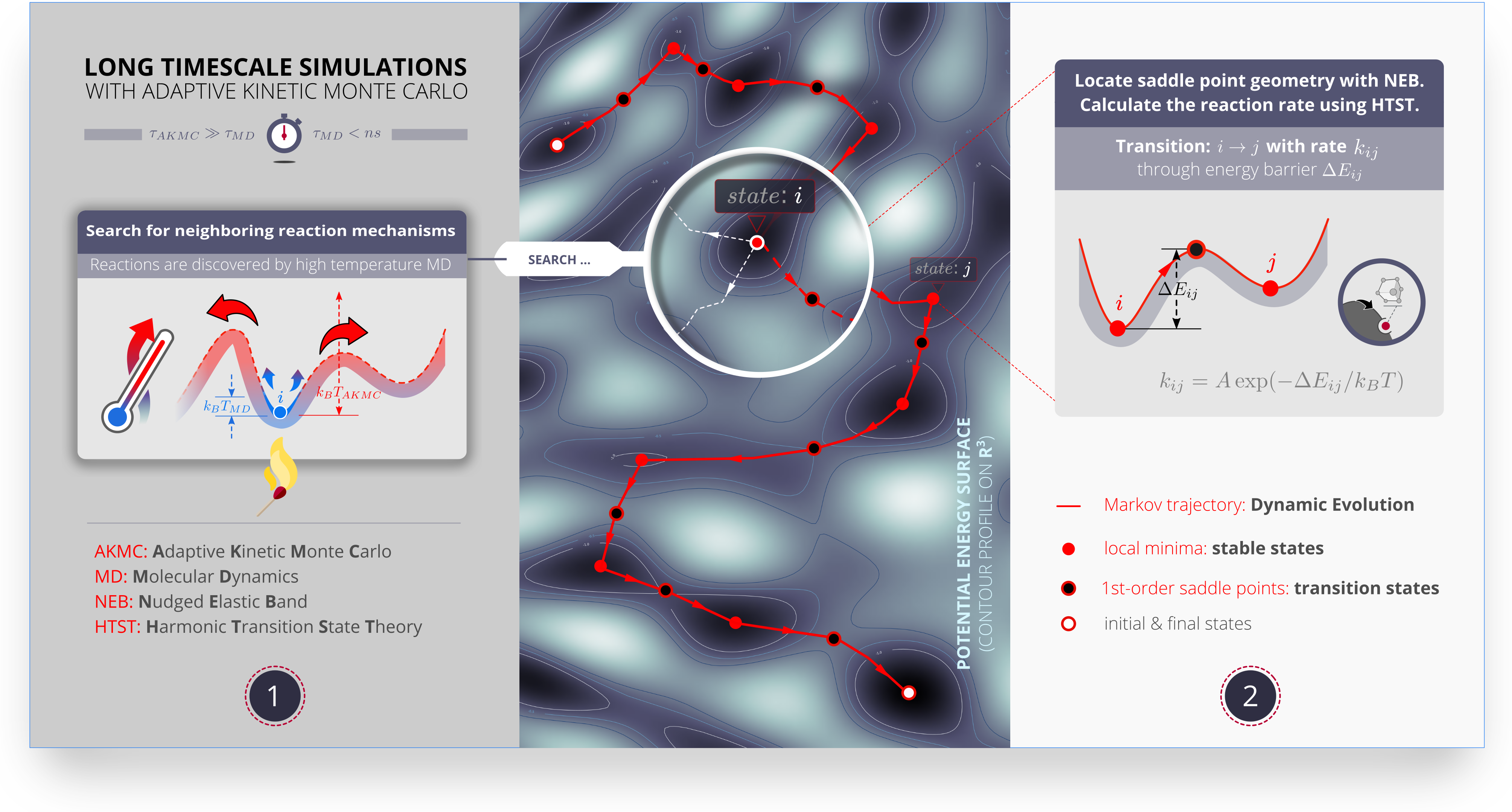

The AKMC method
In solid state systems, atoms reside near their equilibrium positions and reactions are rare events. Because the reactions occur on a much longer timescale than the typical vibrational period of the system (~100 fs), it is not possible to use molecular dynamics (MD) simulations to model solid-state reactions. MD simulations can only routinely access the nanosecond timescale while room temperature solid-state reactions of interest may occur on the millisecond timescale or longer.
Adaptive Kinetic Monte Carlo (AKMC) is a powerful tool for simulating the dynamics of solid-state systems that works by identifying the bottleneck regions between the stable minima and then modeling the reactions between them using statistical mechanics. More specifically, the bottleneck regions are the saddle points on the potential energy surface. These points lie on the minimum energy pathway between two minima, which is the statistically most likely path for a reaction to occur along. The primary computational expense in an AKMC simulation is in locating these saddle points.
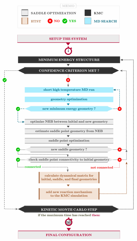
In the AKMC implementation in QuantumATK, the saddle points are located by running high temperature MD trajectories. These trajectories should be hot enough that a few picoseconds of dynamics will be sufficiently long for a reaction to occur. The saddle points are located by periodically minimizing the MD trajectory to detect when the trajectories minimizes to a new geometry. Once the new minimum is located, the saddle point is found by running a nudged elastic band (NEB) calculation.
Once the saddle points are identified, the reaction rates can be estimated using harmonic transition state theory (HTST). In HTST, the reaction rate is given by:
where \(k\) is the reaction rate, \(A\) is the vibrational prefactor, \(ΔE\) is the difference in energy between the saddle point and the minimum (energy barrier), \(k_{B}\) is Boltzmann’s constant, and \(T\) is the temperature.
The HTST rates can then be used to run a kinetic monte carlo (KMC) simulation. In KMC, the system is represented using a Markov chain. Each state of the Markov chain represents a stable state of the system (a local energy minimum) and the transition probabilities between the states are related to the reaction rates (determined from the saddle points). The state of the system is evolved from minimum to minimum. The next state is chosen with a probability proportional to its rate. The amount of time taken to transition to the next state is drawn from an exponential distribution with a rate parameter equal to the total escape rate from the state. When the dynamics are modeled in this way, the computational cost to model one step of the dynamics is very small. Tens of thousands of steps can be performed per second on a typical computer.
For the AKMC simulation to be accurate, it is crucial that the fastest reaction mechanisms are discovered as they represent the most likely events to be chosen in the KMC simulation. To ensure the accuracy of the simulation, each state in the Markov chain has an associated confidence. This confidence is an estimate of the probability that for each KMC step taken from that state, the correct event was chosen. Saddle searches are executed in each state until a user defined confidence level is reached. Once the confidence level is reached, the KMC simulation will proceed until a state is reached where the confidence is less than the target level.
Below is a basic flowchart for the AKMC algorithm. The adaptive part finds saddle points in inner loops. The KMC part updates the total time and the current configuration.
For more details on AKMC and HTST see f.ex. [1] and [2]. For an introduction to KMC see [3].
Creating the initial configuration
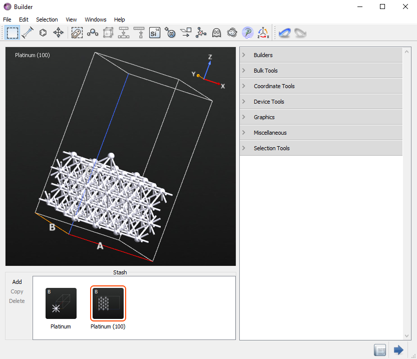
The initial configuration will be a 4 layer p (4x4)-Pt(100) slab with a single adatom occupying a four-fold hollow site.
As the first step, import the Pt fcc bulk configuration by clicking on and search for Platinum. The Pt primitive cell will appear in the Stash.
Click on
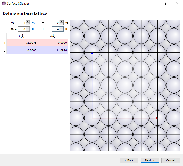
In the new window choose the (100) Miller indices.
Define the p (4x4) surface unit cell.
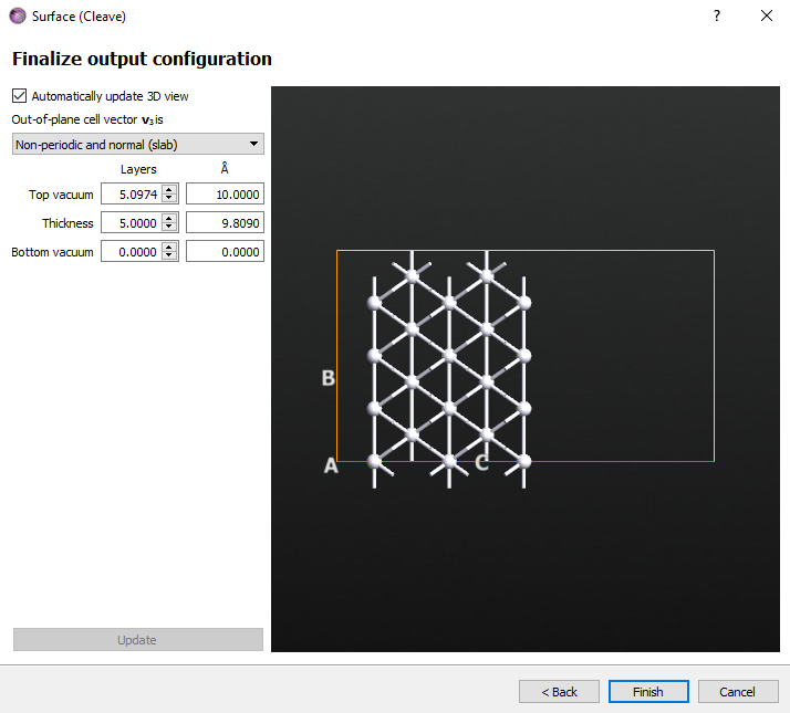
Choose the non-periodic and normal (slab) configuration with five layers, 10 Å of top vacuum. Click Finish.
Your Pt(100) slab is now present in the Stash. The next step is to add the Pt adatom in a four-fold hollow position. Instead of adding a new atom on top of the slab, we will instead delete all but one atom from the topmost layer.
Select three of the four top rows of atoms as shown below and then press the delete key.
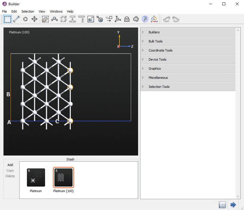
Now rotate the configuration so that the remaining row of four surface atoms is visible. Select three of the four atoms and then press the delete key. The final surface should have just one adatom in a four-fold hollow site.
Creating the AKMC script
Now that we have the initial configuration, we can start the AKMC simulation.
Send the initial configuration to the Script Generator by clicking the
 button.
Add
 New Calculator and
  blocks.
Change the output name to
akmc.nc.Double-click the
New Calculator block and modify the following parameters:Select the ATK-ForceField calculator
Choose the EAM_Pt_2004 Parameter set
In the
OptimizeGeometry block, change the following parameters:Set the maximum force to 0.01 eV/Å
Click the Atomic Constraint Editor button, select the 2 bottom layers, click Add tag from Selection, and change the constraint type from None to Fixed

Now, you will add the AKMC part of the script.
Note
Starting from the ATK 2017 version, you can use the
AdaptiveKineticMonteCarlo block in the Script Generator.
While if you have an older version, you need to follow the below instructions on appending the AKMC code in the editor. Link to 2016 and 2015 versions.
Note
For QuantumATK-versions older than 2017, the ATK-ForceField calculator can be found under the name ATK-Classical.
In the 2017 version, add the object, and double click the AdaptiveKineticMonteCarlo block. You can see the warning for the Atomic Constraint Editor setting. You need to define the atomic constraint again, usually in the same way as in the Optimization, but not necessarily
In Kinetic Monte Carlo, change the confidence to 0.95
In Saddle Search Settings, set the number of searches to 100
Click the Atomic Constraint Editor in the Optimization, select the two bottom layers, change to Fixed for the constraint.
For Nudged Elastic Band, Maximum number of images is 5 and check the Climbing image method
Note
If you need more information to setup the condition, click the Help… button in the Adaptive Kinetic Monte Carlo widget.
If you now send the script to the editor, you will see the following at the end of the script.
# -------------------------------------------------------------
# Adaptive Kinetic Monte Carlo
# -------------------------------------------------------------

saddle_search_parameters = SaddleSearchParameters(
    max_neb_images=5,
    neb_climbing_image=True,
    )

if os.path.isfile('akmc_markov_chain.nc'):
    markov_chain = nlread('akmc_markov_chain.nc')[-1]
else:
    markov_chain = MarkovChain(
        configuration=bulk_configuration,
        configuration_energy=TotalEnergy(bulk_configuration).evaluate(),
        )

if os.path.isfile('akmc_kmc.nc'):
    kmc = nlread('akmc_kmc.nc')[-1]
else:
    kmc = None

constraints = [ 0,  1,  2,  3,  4,  5,  6,  7,  8,  9, 10, 11, 12,
               13, 14, 15, 16, 17, 18, 19, 20, 21, 22, 23, 24, 25,
               26, 27, 28, 29, 30, 31]

akmc = AdaptiveKineticMonteCarlo(
    markov_chain=markov_chain,
    kmc_temperature=300.0*Kelvin,
    md_temperature=2000.0*Kelvin,
    calculator=bulk_configuration.calculator(),
    kmc=kmc,
    saddle_search_parameters=saddle_search_parameters,
    constraints=constraints,
    confidence=0.95,
    filename_prefix='akmc',
    )

akmc.run(max_searches=100, max_kmc_steps=10000)
Note
If you look at the 2017 version of the script, there are two if blocks for repeating runs; it reuses the already completed saddle searches.
In ATK 2016 and ATK 2015, send the script to the  Editor using the Send To icon. Then append the below code to the bottom of the script.
ATK 2016
# -------------------------------------------------------------
# AKMC
# -------------------------------------------------------------
saddle_search_parameters = SaddleSearchParameters(max_neb_images=5)
markov_chain = MarkovChain(bulk_configuration, TotalEnergy(bulk_configuration).evaluate())
akmc = AdaptiveKineticMonteCarlo(markov_chain,
                                 kmc_temperature=300.0*Kelvin,
                                 md_temperature=2000*Kelvin,
                                 calculator=calculator,
                                 saddle_search_parameters=saddle_search_parameters,
                                 write_searches=True,
                                 constraints=fix_atom_indices_0,
                                 confidence=0.95)
akmc.run(100)
ATK 2015
# -------------------------------------------------------------
# AKMC
# -------------------------------------------------------------
saddle_search_parameters = SaddleSearchParameters(max_neb_images=5)
markov_chain = MarkovChain(bulk_configuration, TotalEnergy(bulk_configuration).evaluate())
akmc = AdaptiveKineticMonteCarlo(markov_chain,
                                 kmc_temperature=300.0*Kelvin,
                                 md_temperature=2000*Kelvin,
                                 calculator=calculator,
                                 saddle_search_parameters=saddle_search_parameters,
                                 write_searches=True,
                                 constraints=constraints,
                                 confidence=0.95)
akmc.run(100)
Note
The only difference between the 2016 and 2015 versions is how the constraints are defined.
This code defines an AKMC simulation that will model the dynamics of the system at 300 K (kmc_temperature). The MD saddle searches will be performed at 2000 K (md_temperature). The confidence is set to 95% (confidence).
Save the script as akmc.py and send it to the  Job Manager and run it.
In this case, the calculation will take around 2 hours to complete when run in serial. Additionally, the AKMC simulation can be parallelized using MPI. When run in parallel one MPI process is reserved as the master process that schedules the work. The remaining worker processes are then used to carry out the saddle searches. This means that if two MPI processes are used no speedup will be observed since there will only be one worker process. There should be a linear speedup as the number of MPI processes is increased.
Analyzing the results
Note
Since AKMC is a stochastic method, your results may differ slightly from what is shown here.
Since a large number of files are created during the calculation, it may be useful to click on the list of project files and click Uncheck. But if you uncheck the write searches box in the I/O settings in the AKMC widget or set write_searches = False in the script, fewer files will be written.
Markov Chain Analyzer
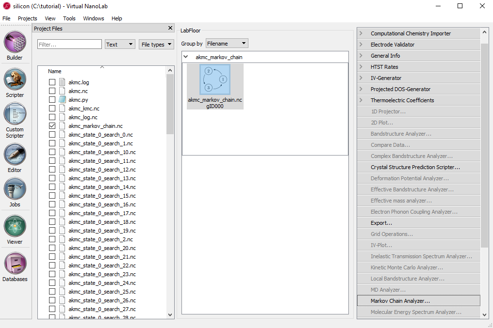
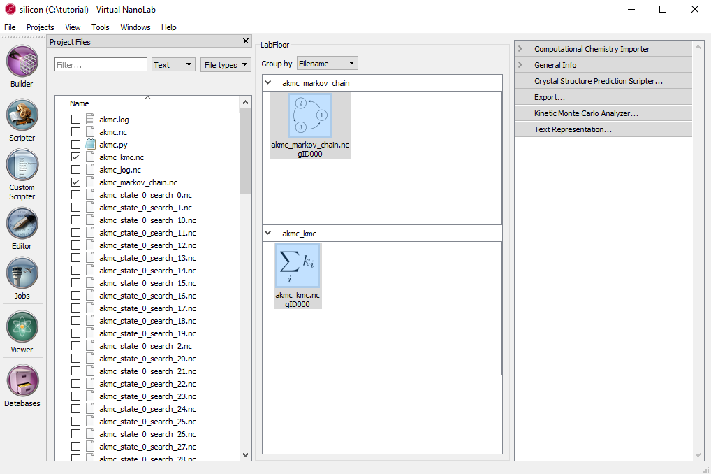
The file akmc_markov_chain.nc contains all of the saddle points and minima that were found during the calculation. Check the box next to the filename to load it onto the LabFloor. Then select it and click on the Markov Chain Analyzer button in the panel.
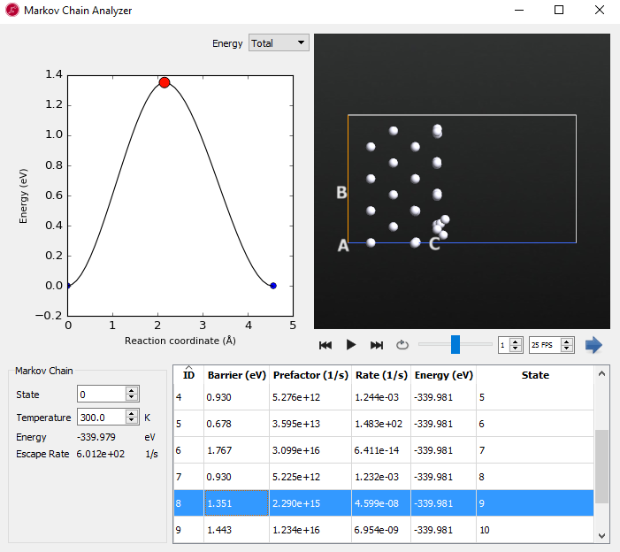
The new window that popped up can be used to examine all of the minima and saddle points that make up the Markov chain.
State 0 is shown in the below table, this corresponds to the initial configuration made at the beginning of this tutorial. By clicking on item in the table, different events can be visualized. In the top left, an energy coordinate diagram is shown for the event and in the top right is a viewer for the trajectory of the minima and saddle point configurations.
For each event, the energy barrier, harmonic prefactor (the variable A in the HTST equation above), reaction rate at the current temperature, and the energy of the final state as well as the state number for the final state are displayed.
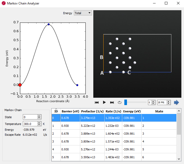
In these results you can see that there are 4 identical reactions with a barrier of 0.678 eV. By using the viewer to look at the saddle point configuration it is apparent that these correspond to the so-called “exchange” mechanism of adatom diffusion where the adatom pushes a surface atom up onto the surface.
This is in contrast to the most obvious diffusion mechanism - the “hop” - where the adatom directly moves to an adjacent four-fold hollow site. The relative rates of these two diffusion mechanisms show that at room temperature the exchange mechanism is the primary way that the adatom diffuses. This is because the rate of the exchange mechanism is 5 orders of magnitude larger than the hop mechanism.
Kinetic Monte Carlo Analyzer
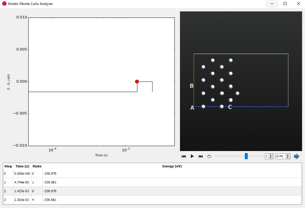
The file named akmc_kmc.nc contains the state-to-state KMC trajectory. Click the checkbox next to the filename to load it onto the LabFloor. Click on its icon and click Text Representation in the panel. The popup window will display the state of the KMC simulation as a function of time. The state number in the right-hand column corresponds to the state numbers in the Markov chain file we just looked at. In this example, the simulation took one step from state 0 to state 1 and 47 microseconds of time elapsed.
# Item:  0
# File:  C:\tutorial\akmc_kmc.nc
# Title: akmc_kmc.nc - gID000
# Type:  KineticMonteCarlo
     Step #   Time (seconds)  State
         0   0.00000000e+00      0
         1   4.74388502e-05      1
         2   1.42688935e-03      0
         3   2.30287130e-03      4
A graphical representation of the KMC trajectory is also available. In order to use it, both the KineticMonteCarlo and MarkovChain objects on the LabFloor must be selected. Then you may click on Kinetic Monte Carlo Analyzer in the panel.
The Kinetic Monte Carlo Analyzer displays the same information shown in the text representation in the table at the bottom of the windows. However, it also makes a plot of the energy versus time and shows the geometry of the currently selected state. Since the energy plot is logarithmic on the time axis the first state at zero seconds cannot be seen, and there are only three data points. The energies are plotted by the difference between the first state 0 and searched state versus time.
AKMC Log
The next file to examine is akmc_log.nc. This file contains a brief summary of the outcome of each of the saddle searches used to find the states shown above. Click the checkbox next to the filename to load it onto the LabFloor. Click on its icon and click Text Representation in the panel.
# Item:  0
# File:  C:\tutorial\akmc_log.nc
# Title: akmc_log.nc - gID000
# Type:  AKMCLog
state id search number confidence  message
       0             0   0.000000  Found new state
       0             1   0.864665  Found saddle connecting to state 1 again
       0             2   0.864657  Found new state
       0             3   0.395535  Found new state
       0             4   0.864661  Found saddle connecting to state 3 again
       0             5   0.564633  Found new state
       0             6   0.564631  Found new state
       0             7   0.590186  Found saddle connecting to state 1 again
       0             8   0.590186  First order saddles have exactly one negative frequency, not 2 negative frequencies.
       0             9   0.590188  Found saddle connecting to state 5 again
       0            10   0.590188  First order saddles have exactly one negative frequency, not 2 negative frequencies.
       0            11   0.444580  Found new state
       0            12   0.670587  Found saddle connecting to state 4 again
       0            13   0.670587  First order saddles have exactly one negative frequency, not 2 negative frequencies.
       0            14   0.670587  First order saddles have exactly one negative frequency, not 2 negative frequencies.
       0            15   0.670587  First order saddles have exactly one negative frequency, not 2 negative frequencies.
       0            16   0.692947  Found saddle connecting to state 4 again
       0            17   0.700029  Found saddle connecting to state 1 again
The output above shows the first 17 lines of output. Each line corresponds to a single saddle search.
The state id column represents the id number for the state that the saddle searches are started from. The search number is unique identifier for each search. The confidence represents an estimate of the confidence in the KMC simulation for the state. The confidence is used as the stopping criteria for the saddle searches. The message column summarizes the result of the saddle search.
The message Found new state means that a new reaction mechanism was discovered. The message Found saddle connecting to state 1 again means that a previously discovered saddle point was found.
There are a number of possible error messages that can occur. In this case the message First order saddles have one negative frequency not 2 negative frequencies means that a saddle point was found, but when the vibrational modes were calculated more than one negative frequency was identified. There could be a number of reasons for this issue. Often times classical potentials are not fit near saddle points and can have unexpected behavior.
Diagnosing Errors
When there is an issue with a saddle search, an error message will be displayed in the log. The state id and search number columns can then be used to locate a file with more information about the search, if the parameter write_searches=True was passed to the AdaptiveKineticMonteCarlo class. In this case we look at search number 1. The filename is akmc_search_0_search_1.nc. Remember, in your simulation the numbers may be different. Click the checkbox by the filename of akmc search you wish to inspect. Then you can click on the Optimized NEB item and then click on Movie Tool in the panel to visualize the reaction pathway.

In general, if it was lower energy barrier, it will be an important reaction path. But in this case, we see that this is another type of exchange diffusion mechanism even higher in energy than the hopping mechanisms that we already showed was too slow to contribute to adatom diffusion.
By using the Movie Tool in the Markov Chain Analyzer, we can examine each state to understand the diffusion mechanism.
In a real study it is always important to verify the results of a classical potential and re-optimizing this NEB using DFT would be a good idea to determine if it was a real pathway in the system.
Conclusion
In this tutorial we examined how to construct a Pt(100) slab model with a single adatom. We then performed an AKMC simulation to model the diffusion of the adatom at 300 K. The results showed two different diffusion mechanisms: the exchange and hop processes. The exchange process was found to be the dominant mechanism for adatom diffusion.
This simulation was a very simple case. No matter how the adatom diffuses the system is the same by symmetry (i.e. the adatom will always have the same set of 4 exchange and 4 hop diffusion mechanisms). So once one state has been explored, there is nothing left to learn. However, in the current implementation, the AKMC code does not take symmetry into account and must do saddle searches for each new state. Most systems of interest do not contain such high levels of symmetry.