Reconstruction of the Si (100) surface - a geometry optimization study with QuantumATK
Introduction
Although LDA and GGA may not be able to produce a proper band gap in Si (and most other semiconductors), these “simple” DFT functionals are very capable when it comes to predicting geometrical properties. In this short tutorial we will demonstrate how to use QuantumATK to study the so-called asymmetric dimer reconstruction of a Si (100) surface.
The focus will be on the physics and how to set up the model correctly, rather than how to operate QuantumATK. It will be assumed that you have experience building structures (for instance, cleaving surfaces) and setting up calculations and inspecting the results, and the steps will therefore only be indicated, not explained in any great detail.
Building the geometry
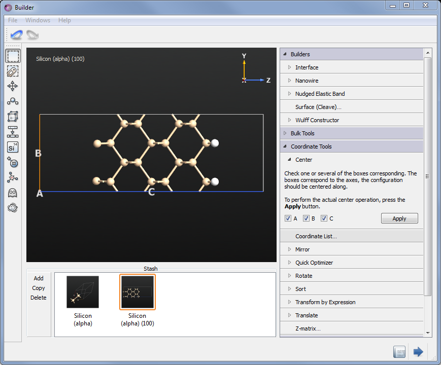
Start QuantumATK and open the Builder.
Add Silicon (alpha) from the Database ().
Open .
Cleave the structure along 100 by entering the corresponding Miller indices.
Since the dimer reconstruction can only occur in a 2x1 supercell, you need to make a larger surface cell than the smallest one. Therefore, on the second page set \(\mathbf{v_2} = 2\mathbf{u_2}\).

On the final page of the Surface tool, choose a Slab configuration with thickness 4.5 layers (the default size of the vacuum is fine).

Center the structure in all directions ().
Select the two Si atoms with the smallest Z-coordinate and add a small random perturbation to their positions by clicking the
Rattletool a few times. This is because the completely symmetric state is a meta-stable configuration, and it’s best to not start the optimization in such a state.
Select the two Si atoms with the highest Z-coordinate and passivate them
 to
saturate all Si bonds in the structure.
to
saturate all Si bonds in the structure.
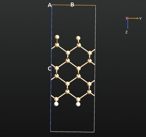
The resulting structure is shown in the picture below.
Setting up the calculation
Send the structure to the ScriptGenerator.
Insert a New Calculator block, then an OptimizeGeometry block.
For the calculator you can keep all parameters at their default except the k-point sampling. Set it to 9x9 (of course 1 point is enough in the C direction, since it’s a slab) - accuracy is important since the difference in energy between the symmetric and asymmetric dimer states is very small [1].
For the optimization, constrain the two bottom Si atoms and the 4 hydrogens. It is always important to limit the degrees of freedom in a relaxation if possible, to project out pure translations and rotations.
Also, make sure to tick
Save trajectoryand set a name for the trajectory file.
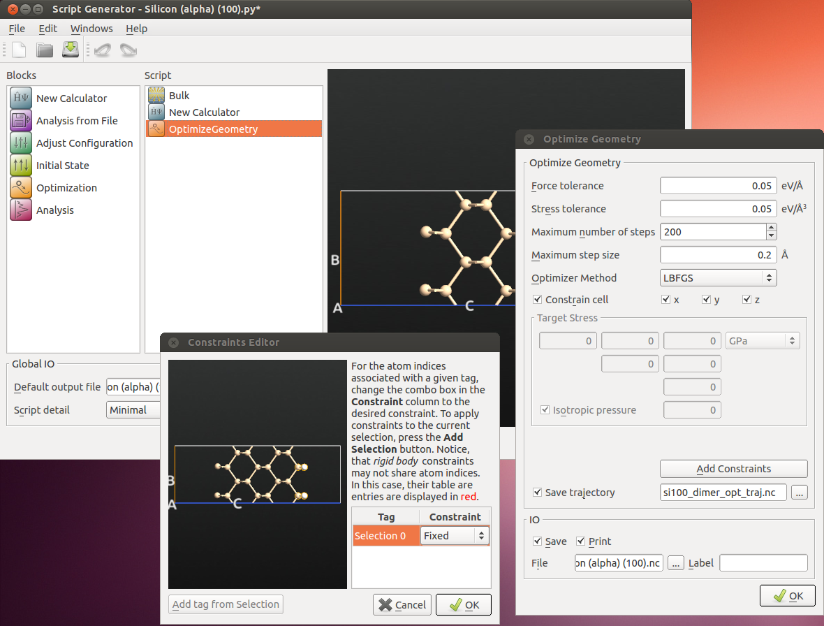
Set the name of the output file, and the calculation is ready to be run. Save the script!
Send the script to the Job Manager, or transfer it to a cluster and run it there. This calculation parallelizes very well, and takes between one and several hours depending on how many MPI nodes it is run on.
Results
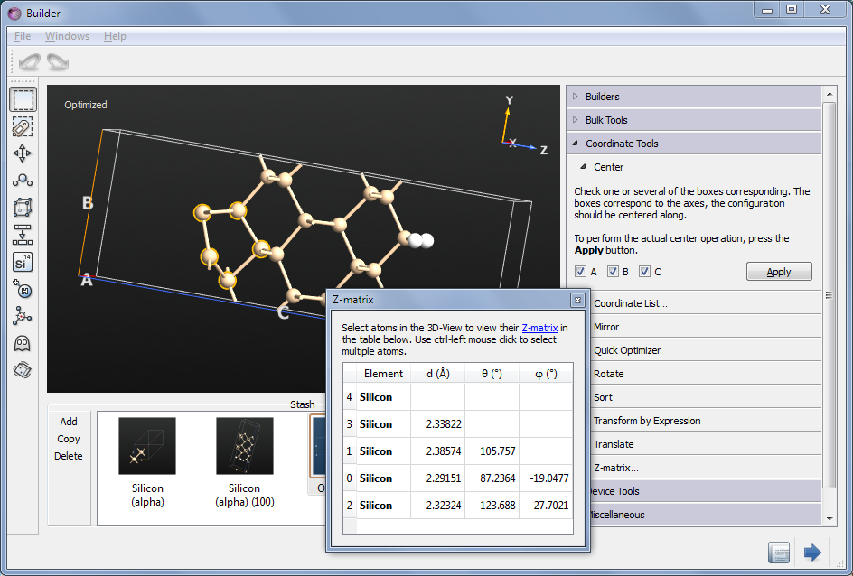
When the calculation is done, select the HDF5 file in QuantumATK and inspect the second “Bulk configuration”, with Id “gID001” - this is the optimized geometry.
Drag-and-Drop it on the Builder - it is immediately visible that indeed an asymmetric dimer state has been obtained. To display the bond lengths just hoover the mouse over the respective bond - the bond distance will be displayed in the tool tip. To perform measurements of the bond lengths and angles, open , and select various atoms in the surface - both for the original and optimized geometry - and compare.
It is also interesting to analyze the relaxation trajectory. Select the LabFloor object in which you have the saved the trajectory, and open it in the Viewer to watch a movie of the optimization.
If we plot the total energy and forces for each relaxation step, we see that the total energy is more or less constantly decreasing, as expected from the fact that we use the LBFGS algorithm, which indeed is designed to minimize the total energy rather than just following the forces. The following simple script reads the trajectory data and plots the total energy and maximum force for each step:
traj = nlread('si_100_traj.hdf5', Trajectory)[0]
energies = []
max_forces = []
for i in range(len(traj)):
    energies.append(traj.imageEnergy(i).inUnitsOf(eV))
    forces = traj.imageForces(i).inUnitsOf(eV/Angstrom)
    force_magnitude = (forces**2).sum(axis=1)**0.5
    max_forces.append(numpy.max(forces))

# Plot the energy and max. force curve using pylab.
import pylab

pylab.figure()
pylab.subplot(2, 1, 1)
pylab.plot(range(len(traj)), energies)
pylab.xlabel('Optimization step')
pylab.ylabel('Energy (eV)')
pylab.grid(True)

pylab.subplot(2, 1, 2)
pylab.plot(range(len(traj)), max_forces)
pylab.xlabel('Optimization step')
pylab.ylabel('Maximum Forces (eV/Ang)')
pylab.grid(True)

pylab.show()
The result may look like the figure below, although the exact curve depends on the exact initial displacement of the top silicon atoms.
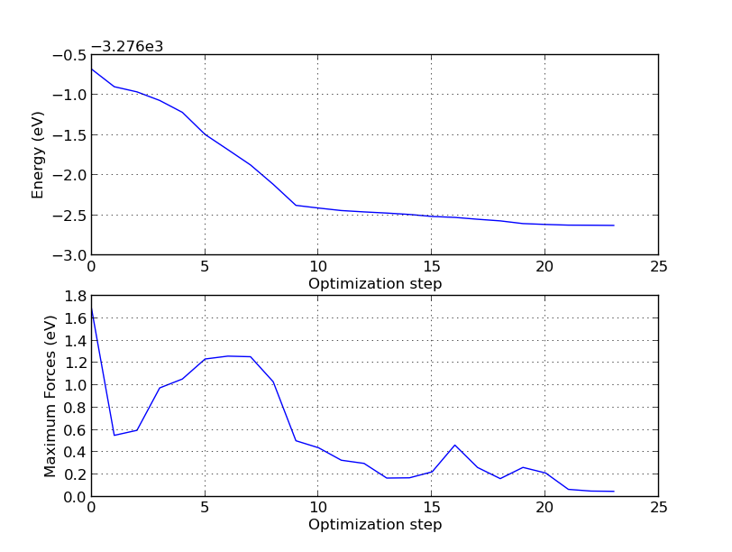
From this plot, combined with the trajectory movie, you can learn many things. First of all, note that unless you use a criterion for the forces which is below 0.2 eV/Å, you would be fooled into thinking the symmetric dimer is the minimum, since this state is passed on the way to the asymmetric one! This is also possible to see in the trajectory movie. In fact, although it has not been shown here, it is well known that unless care is taken to have an accurate method (i.e. enough k-points) and even enough vacuum around the slab, the symmetric dimer will be predicted to be the most energetically favorable.
Specifically, the symmetric dimer local minimum is reached around step 13 (see the trajectory picture above), but as the algorithm tries to reduce the total energy further, the forces rise again and the asymmetry starts to appear. After step 15 an asymmetry has been established for real, and the asymmetric dimer is finally formed at around step 20.
You can use the following script to visualize the vertical relaxation of the atomic layers:
traj = nlread('si_100_traj.hdf5', Trajectory)[0]
number_of_steps = len(traj)
z_coordinates = []

for i in range(number_of_steps):
    coordinates = traj.image(i).cartesianCoordinates().inUnitsOf(Angstrom)
    # Append all z-coordinates, apart from the fixed bottom layer.
    z_coordinates.append(coordinates[:16, 2].tolist())

# Convert to numpy array.
z_coordinates = numpy.array(z_coordinates)
# Plot the z-coordinates using pylab.
import pylab

pylab.figure()
# Loop over all unconstrained atoms.
for i in range(16):
    pylab.plot(range(number_of_steps), z_coordinates[:, i], '--*')
pylab.xlabel('Optimization step')
pylab.ylabel('Z-coordinates (Ang)')
pylab.grid(True)

pylab.show()
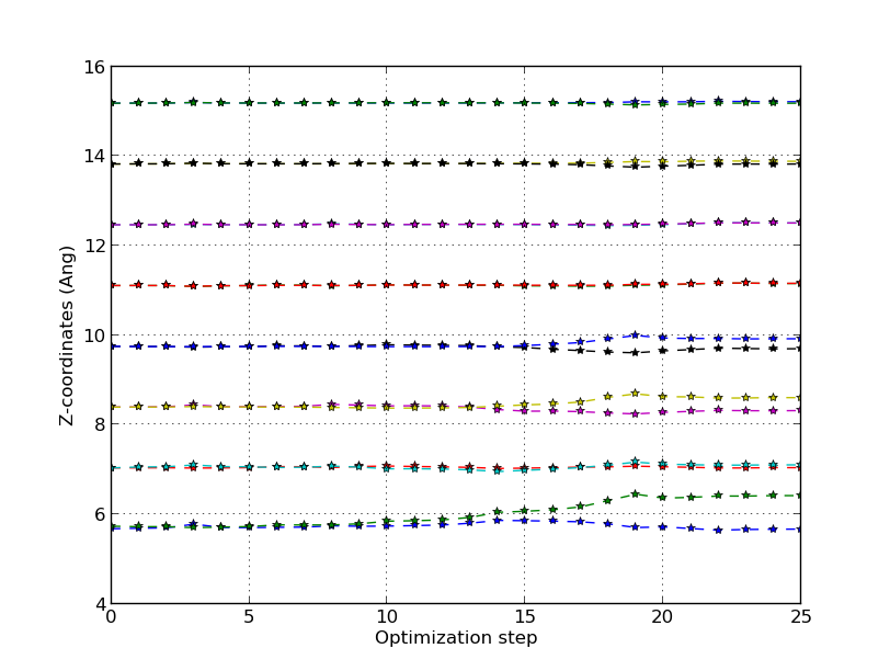
It is important to note that the asymmetry appears as a result of a long-range interaction, which also is why short-range methods like tight-binding or classical potentials are only able to relax the configuration into the symmetric dimer.
Summary
This study has shown how QuantumATK can succesfully predict even a rather complicated geometric reconstruction by using geometry optimization in DFT. The Si 100 surface first forms a symmetric dimer which in turns induces an asymmetry in the electron landscape, under which we again optimize the structure to find the ground state asymmetric structure. The asymmetry is a long-range effect which originates a few layers below the surface where the Si lattice is compressed downwards under the dimer.
References