Finding Transition States

Finding transition states and thus reaction barriers is a key application of in ab-initio atomistic modelling. Knowing the transition state allows the calculation of reaction rates and gives qualitative insight into the mechanism of chemical reactions, diffusion processes, and phase transitions. Unfortunately, obtaining tightly converged transition states can be challenging, and often requires a lot of computational resources and human expertise.

QuantumATK provides state-of-the-art algorithms and graphical tools to make the process of setting up, running, and analyzing transition state calculations as intuitive and efficient as possible. This document provides an overview of the available methods and gives recommendations on how to use them.

Nudged Elastic Band

The NudgedElasticBand (NEB) method is a widely used technique to find transition states. It is a double-ended method, meaning that it requires the user to provide the initial and final states (i.e. the reactants and products) of the system. The NEB method then finds the minimum energy path (MEP) connecting these states with a chain of images. The images are relaxed to the MEP with the highest energy image being usually a good approximation of the transition state.

This approximate transition state can then be used as a starting point for more accurate or more efficient methods to refine towards the actual transition state (see Minimum mode following techniques).

Setting up the NEB Configuration

The easiest way to set up an NEB configuration is to use Nudged Elastic Band builder in NanoLab.

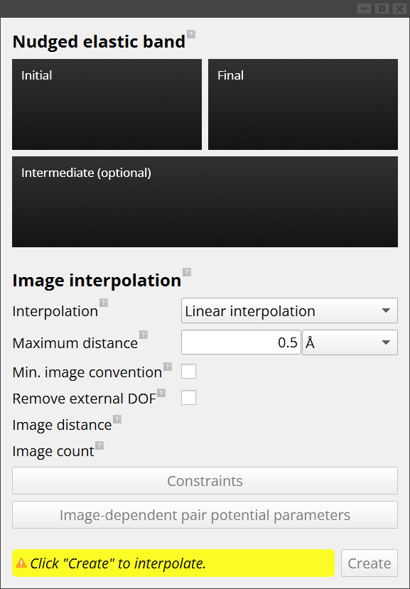
The initial and final states as well as one optional intermediate state can be dropped into the builder from the stash. The NEB can be created with the click of a button. If necessary, some parameters can be adjusted to change the quality of the initial path. The ImageDependentPairPotential is a good general purpose interpolation method, while the SequentialImageDependentPairPotential can be used for more complex reactions. If neither of these converge to an acceptable path, the LinearInterpolation is a fallback option. Remove external degree of freedom to minimize rotations and translations of molecules. The minimum image convention is useful to account for periodic cells.

Optimizing the Path

Optimizing the path is done using the OptimizeNudgedElasticBand function which implements the all-images-optimized algorithm where the whole path is optimized at once. This means that the highest parallel efficiency is achieved when the number of images is equal to the number of processes. Please refer to the documentation of the function for more details.

The AutomaticNEB method is an alternative to the regular NEB optimization which is more efficient at finding the transition state, as it optimizes the path segment by segment. This is especially useful for users who are not able to run many processes in parallel. One downside is that the path is not fully converged, except for the region around the transition state which is refined at the end of the calculation.

NEB Optimization Analyzer

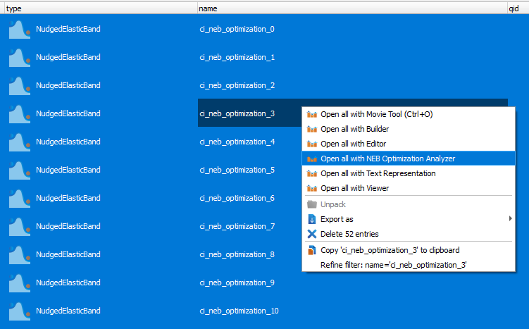
The NEB optimization analyzer is opened from the Data View by selecting multiple NEB objects and right-clicking on one of them. Then select “Open all with NEB Optimization Analyzer”.

The analyzer shows all the relevant information, such as the energy and forces of each image throughout the optimization at a glance. Different tabs are available to drill down into the details of the optimization.

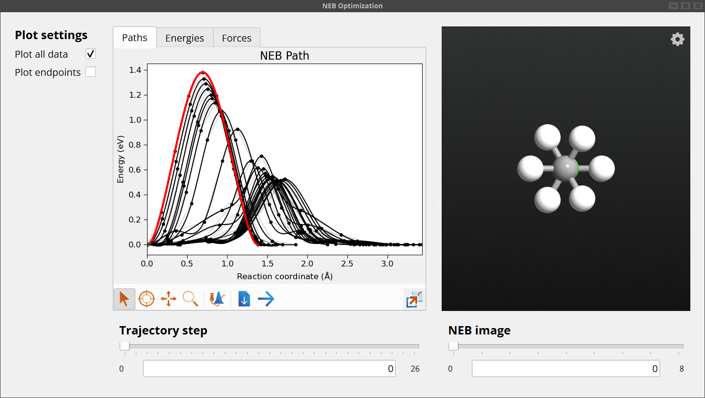
The analyzer is useful for monitoring the convergence of the NEB optimization and for troubleshooting problems. Some common issues to look out for are:

• Additional minima appearing in the path. It is usually a good idea to separate the path into segments and optimize them individually. For this the split method of NudgedElasticBand can be used. It takes the indices of the images at which to split the path.

• All images are not converging and forces remain high. This is often accompanied by the reaction coordinate becoming longer or energies of images crossing over. Refer to the troubleshooting section of OptimizeNudgedElasticBand() for more information.

• If only a single image is not converging, one might try to switch from NEB to a different method (see Minimum mode following techniques).

Minimum Mode Following Techniques

Minimum mode following techniques are a class of methods that start from a single configuration and follow the smallest eigenmode to search for nearby transition states. This can be advantageous in cases where the initial and final states are not known. Another common application is to refine the transition state found by the NEB method.

Two popular minimum mode following techniques are the Dimer and the Lanczos method. The Dimer method uses a finite difference approximation of two images (hence the name) displaced from the current configuration along the eigenmode and rotations around the axis of displacement to estimate the smallest eigenmode. In this way it avoids the expensive calculation of the Hessian matrix. The Lanczos method is conceptually similar to the Dimer method and differs mainly in the way the smallest eigenmode is estimated. It uses an approximate Hessian that is systematically built up during the optimization.

As both methods use finite differences they can be sensitive to noise in the forces. It is recommended to use a force field with smooth forces or DFT calculators with a tighter SCF tolerance. Generally speaking, both methods have similar performance characteristics overall [1] and are more efficient than the NEB at locating an exact transition state when more than 5-6 images are used for the NEB.

Best Practices and Recommendations

Transition states often require a tighter force tolerance than minima to satisfy the condition of exactly one imaginary frequency. A force tolerance of 10**-3 ev/Ang is usually sufficient, but it is good practice to calculate the vibrational spectrum using the VibrationalMode analysis object. This additional step is crucial to get accurate barrier heights since errors scale quadratically.

Usually, finding a transition state is a multi-step process involving several of the methods listed above. A common workflow might look like this:

1. Start with pre-converging the NEB using the default force tolerance and, optionally, a larger number of images.

2. Re-run the NEB optimization with a tighter force tolerance and fewer images while turning on the climbing image option. This will push the highest energy image towards the transition state. If the reaction is relatively simple, steps 1 and 2 may be combined.

3. Refine the transition state using the Dimer or Lanczos method with the final force tolerance. Here, the initial search direction can also be extracted from the NEB path using dimerFromNEB.

A convenient way to automate the search for transition states is to use the automaticTransitionState function.

It is generally advisable to use an odd number of images to ensure that the transition state is in the middle of the path.

References

[1]

R. A. Olsen, G. J. Kroes, G. Henkelman, A. Arnaldsson, and H. Jónsson. Comparison of methods for finding saddle points without knowledge of the final states. The Journal of Chemical Physics, 121(20):9776–9792, 11 2004. URL: https://doi.org/10.1063/1.1809574, arXiv:https://pubs.aip.org/aip/jcp/article-pdf/121/20/9776/19220457/9776\_1\_online.pdf, doi:10.1063/1.1809574.