Simulating a creep experiment of polycrystalline copper
Version: 2016.3
This tutorial will show how to set up, run, and analyze a molecular dynamics (MD) simulation of a microscopic creep experiment using polycrystalline copper, i.e. the strain response to an externally imposed uniaxial stress [1]. You will get to know the Polycrystal Builder and the Local Structure analysis tool, and you will learn how to run advanced MD simulations at constant external stress.
Although the construction of realistic grain sizes of several nanometers is in principal possible, the computational cost of such simulations is relatively large, as the required system size can easily exceed a million atoms. Such calculations are certainly possible with QuantumATK, but for demonstration purposes you will here simulate only a small model system, to reduce the calculation time. Still, the presented methodology can be transferred in a straightforward manner to larger systems.
Installing the polycrystal builder plugin
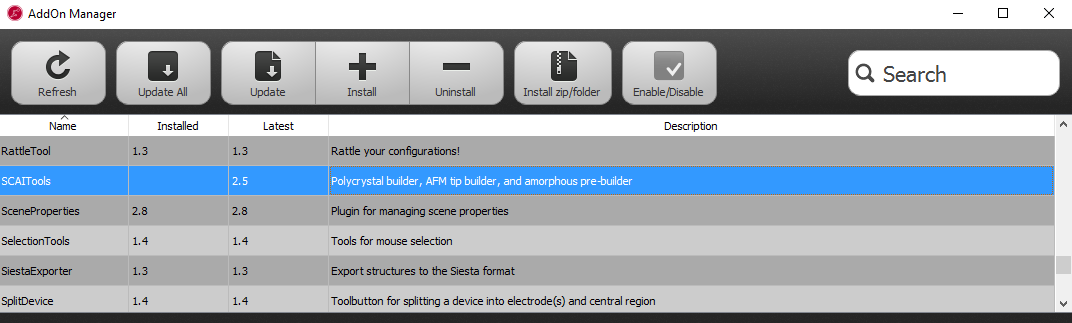
First, make sure that the Polycrystal plugin is installed and available in the Builder – it should appear in the Builder panel under . If the plugin is not listed, you have to install it via . Select the SCAITools package and install it.
You may have to restart QuantumATK to activate the plugin in the Builder.
Building the polycrystalline cell
Create a new project in QuantumATK, call it for instance “Polycrystalline Copper”.
Open the  Builder and add the fcc copper single crystal
material to the Stash using .
Builder and add the fcc copper single crystal
material to the Stash using .
To start building the polycrystalline structure, select . Set the crystal size to 50, 50, 50 Å to obtain an cubic supercell. Set the gap between grains to a small value, like 0.1 Å, to allow for a compact packing of the grains. Drag and drop the cubic copper cell from the Stash to the Materials field. Make sure the Generate grain based tags option is unticked. As an advanced analysis feature, this option allows you to mark the atoms within each grain by different tags, so that the transformation of the grains during the simulation can be monitored. We will not use this feature in this tutorial.
You can choose how the seeds for the grains are created. Select Generate from superlattice and set the number of grid points to 4. Select FaceCenteredCubic as the superlattice of the grain structure, and set the value of Jitter to 8 Å. These settings will create four initial grains on a distorted fcc lattice, with a distortion variance of 8 Å.
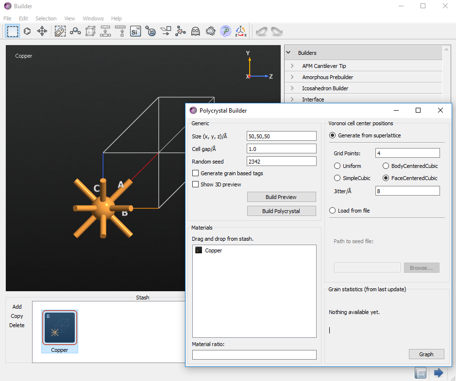
You can preview the grain structure by clicking Build Preview. Now, the 3D-window will show the only the seeds of the grains. You can additionally switch on the visualization of the grain boundaries by checking Show 3D preview box.
Click Build Polycrystal to initiate the structure generation.
After a few seconds the final polycrystalline cell will appear on the Stash.
Analyzing the grain structure
By rotating the cell in the Builder window, you can already see part of the grain structure. A better visualization in terms of the local crystal structure can be performed by using the LocalStructure analyzer.
For this, send the polycrystalline cell to  Scripter, and just left double-click
  Analysis and add
the LocalStructure (do not add any New Calculator, as you may be used to
– we are not going to run any simulation, only analyze the real-space
geometry). Change the output filename to something suitable, e.g.
Analysis and add
the LocalStructure (do not add any New Calculator, as you may be used to
– we are not going to run any simulation, only analyze the real-space
geometry). Change the output filename to something suitable, e.g.
local_structure_init.hdf5.
Send the script to the  Job Manager and run it.
After a few seconds, the results will appear on the LabFloor. Select the
LocalStructure item and click the  Viewer. You can now use
the Local Structure plugin in the Viewer to analyze the crystal structure.
You will there find a list of the crystal structure types which have been
detected in the polycrystalline cell.
Viewer. You can now use
the Local Structure plugin in the Viewer to analyze the crystal structure.
You will there find a list of the crystal structure types which have been
detected in the polycrystalline cell.
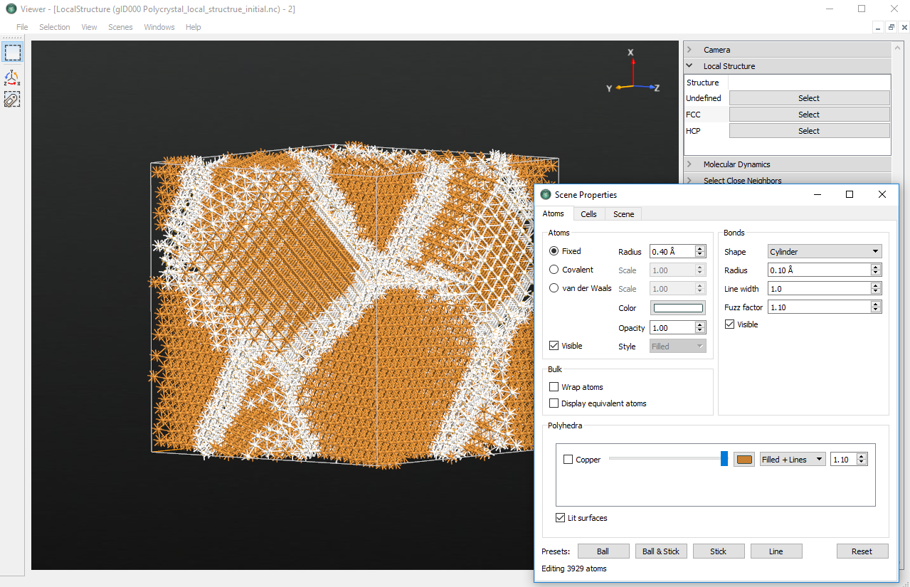
In this example, the cell contains atoms in a local “FCC”, as well as “HCP”, or “Undefined” environment. Since the underlying basic copper crystal forms a fcc strucure, the grains will be of such struture, too. To identify the grain boundaries, click to select all Undefined and HCP atoms (the latter will be only a tiny fraction). Then open the Properties plugin and change the color of the selected atoms to e.g. white. Grains as well as grain boundaries will now be clearly visible, as illustrated above.
Tip
Alternatively, you could uncheck the Visible box to hide the selected grain-boundary atoms, or perform any other customized graphical modification of the scene.
Note
The exact grain structure has been generated randomly and might be different from case to case.
Setting up the creep simulation
You will now set up the MD simulations; first equilibration and then the
actual creep simulation. Send the bulk configuration from the
Builder to the Scripter.
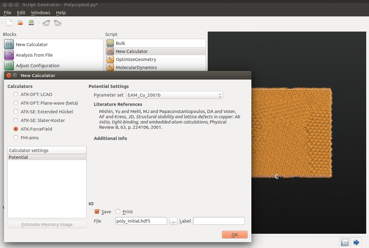
Add a  New Calculator and open it (double-click). Select
ATK-ForceField in the left panel; the suggested Embedded Atom Model (EAM)
potential named EAM_Cu_2001b [2] is a suitable choice. Set
the filename to
New Calculator and open it (double-click). Select
ATK-ForceField in the left panel; the suggested Embedded Atom Model (EAM)
potential named EAM_Cu_2001b [2] is a suitable choice. Set
the filename to poly_initial.hdf5 to save the initial supercell in a
separate HDF5 file – using separate data files can help organize the data.
Uncheck the Print tick box at the bottom to not clutter the log file too
much. Click OK to close the Calculator dialog.
Note
For QuantumATK-versions older than 2017, the ATK-ForceField calculator can be found under the name ATK-Classical.
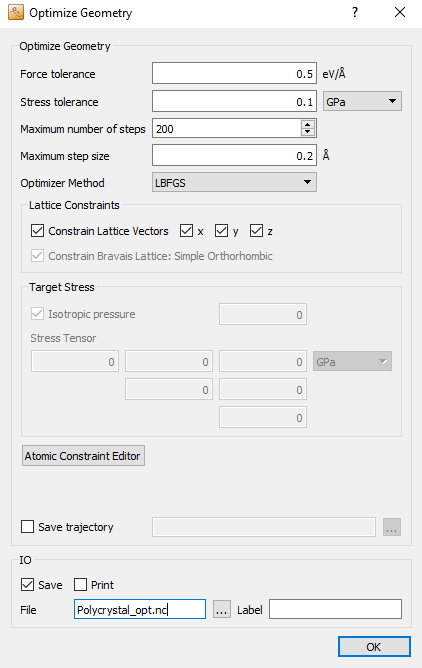
Next, add the  OptimizeGeometry block (click
). This step will remove
possibly large inter-atomic forces due to the building procedure, before
running the actual MD simulation. Double-click to open its settings. As we do
not require a perfectly force-free structure, the force tolerance can be
increased to 0.5 eV/Å, in order to speed up the calculation. The remaining
parameters can be kept at their default values, although you could remove the
checkmarks for Save and Print.
OptimizeGeometry block (click
). This step will remove
possibly large inter-atomic forces due to the building procedure, before
running the actual MD simulation. Double-click to open its settings. As we do
not require a perfectly force-free structure, the force tolerance can be
increased to 0.5 eV/Å, in order to speed up the calculation. The remaining
parameters can be kept at their default values, although you could remove the
checkmarks for Save and Print.
After the geometry optimization, you will want to run two short NVT (constant
volume) and NPT (constant pressure) molecular dynamics simulations to get an
equilibrated configuration. Therefore, add two
MolecularDynamics blocks (click ). Later on, you will add one more MD block for the creep
simulation.
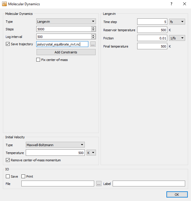
In some cases, in particular if the initial configuration is far from equilibrium, directly starting with a constant pressure simulation can make the system to unstable and lead to unreasonable results. A safer approach is to equilibrate the system at constant volume first, before switching on the pressure coupling. To this aim, select Langevin for NVT simulation in the setting of the first MolecularDynamics block, choose the Maxwell-Boltzmann initial velocities at a temperature of 500 K. You can use a large time step of 5 fs for copper, as the atoms are quite heavy and thus the vibrational frequencies are small enough. Be aware, however, that a time step this large might in other cases affect the accuracy of the integration algorithms, so before simulating a new system one should carefully assess the chosen time step by monitoring the energy conservation in an NVE simulation at the desired temperature.
Set both the reservoir temperature and the final temperature to 500 K. We run the simulation at a slightly elevated temperature to accelerate possible thermally activated processes, to see at least the onset of the creep behaviour in a relatively short simulation time.
Save the trajectory to the file polycrystal_equilibrate_nvt.hdf5.
Uncheck the Save and Print boxes at the bottom, as the trajectory is
already being saved.
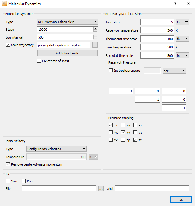
In the next MolecularDynamics block, you will perform another
equilibration simulation, this time at constant pressure. Therefore, select
NPT Martyna Tobias Klein MD type, as this method allows to impose an
independent pressure coupling to each component of the stress tensor. Set the
number of steps to 10,000 and the log interval to 500. Select an
appropriate filename for the trajectory file, e.g.
polycrystal_equilibrate_npt.hdf5.
Choose Configuration velocities as initial velocities.
Choose again a fairly large time step of 5 fs and 500 K for the reservoir and final temperatures. Moreover, make sure that the reservoir pressure is 1 bar.
Uncheck Isotropic pressure to couple each cell vector independently to the barostat. In the field named Pressure coupling you can select which components of the stress tensor the barostat should couple to. Here, you should stick to the default settings, which activate only the hydrostatic stress, without any shear stress components.
Now, for the actual creep simulation, add a third
MolecularDynamics block. Choose the same settings as in the previous (NPT)
MD block, except for the number of steps and the log interval, which
should be set to 40,000 and 250, respectively.
The essential point of a creep simulation is exposing the system to a large uniaxial stress \(\sigma_\mathrm{creep}\) and monitoring the strain response, as illustrated below:
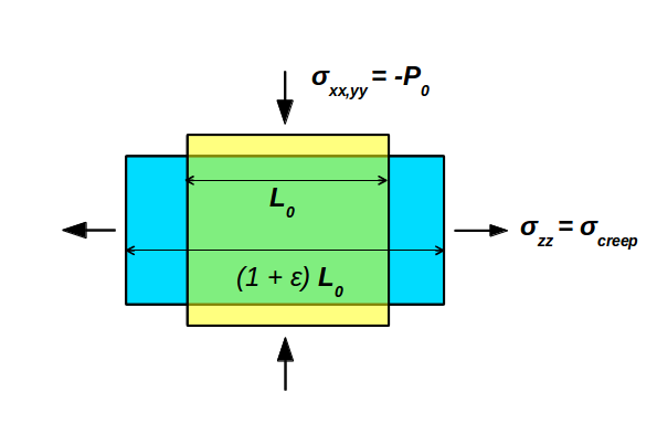
To this aim, you first need to uncheck the Isotropic pressure box, to achieve an independent pressure-coupling of the cell vectors. Then, you need to modfiy the “Reservoir pressure” tensor. The first two diagonal entries (xx and yy) define the ambient pressure perpendicular to the creep direction to allow for lateral relaxation, according the the poisson ratio of the material. For the actual creep stress, which is specified as the third diagonal entry (zz), we set a value of -15,000 bar, corresponding to -1.5 GPa. Note, that negative pressure values are interpreted as tensile external stress.
The off-diagonal entries denote the shear stresses (yz, zx, xy), which do not play a role here as we have de-ativated the coupling to these contributions.

Finally, add another LocalStructure analysis block in
order to be able to analyze and visualize the final grain structure. Open the
block and change the output filename to local_structure_final.hdf5.
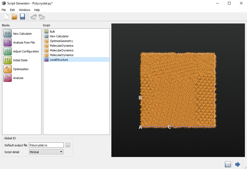
The Script Generator should now look like below.
Send the script to the  Editor by using the
  botton.
Strain vs. time
A creep simulation is commonly analyzed in terms of the strain as a function of time, to measure the response to the imposed stress. To perform a similar analysis for our model simulation you have to add some more lines to bottom of the script you just produced.
These extra QuantumATK Python script lines are shown below and can be downloaded as a
separate script: analysis.py. The relevant data (i.e. cell
vectors, stress, potential energy) are extracted from the md_trajectory
object by using the corresponding class methods. Plots of strain, stress and
potential energy are then plotted using the pylab module, and saved as PNG
files. This analysis can also be carried out separately, after loading a saved
HDF5 trajectory using the nlread() function.
In the Editor, copy the analysis script lines into the bottom on the simulation script.
# -------------------------------------------------------------
# Custom Analysis
# -------------------------------------------------------------
md_trajectory = nlread('polycrystal_creep.nc')[-1]
# Extract the times, cell vectors, potential energies, and pressure tensors
times        = md_trajectory.times().inUnitsOf(picoSecond)
cell_vectors = md_trajectory.cells()
e_pot        = md_trajectory.potentialEnergies().inUnitsOf(eV)
pressure       = md_trajectory.pressureTensors().inUnitsOf(GPa)
# Convert the tensor elements into lists
strain_xx = cell_vectors[:, 0, 0]/cell_vectors[0, 0, 0] - 1.0
strain_zz = cell_vectors[:, 2, 2]/cell_vectors[0, 2, 2] - 1.0
pressure_zz = pressure[:, 2, 2]
# Plot the data usig pylab
import pylab
# Plot the strain
pylab.figure()
pylab.plot(times,strain_zz,'b')
pylab.plot(times,strain_xx,'g')
pylab.title('Creep strain in Copper Polycrystal at 500K and a load of 1.5 GPa')
pylab.xlabel('MD time (ps)')
pylab.ylabel('Strain')
pylab.grid(True)
pylab.savefig("CreepStrain.png")
# Plot the pressure
pylab.figure()
pylab.plot(times,pressure_zz,'b')
pylab.title('Stress in Copper Polycrystal')
pylab.xlabel('MD time (ps)')
pylab.ylabel('Stress (GPa,bar)')
pylab.grid(True)
pylab.savefig("CreepStress.png")
# Plot the potential energy
pylab.figure()
pylab.plot(times,e_pot)
pylab.title('Potential energy during creep in copper polycrystal')
pylab.xlabel('MD time (ps)')
pylab.ylabel('Potential energy (eV)')
pylab.grid(True)
pylab.savefig("CreepEPot.png" )
Running the simulation
After editing the simulation script as desribed above, use the
button to transfer the script to the Job Manager, then
save the script as run_polycrystal.py and run it. The whole simulation
takes approximately an hour, depending on your computing infrastructure, since
the system is quite large (and yet small compared to the geometries studied in
[1]).
Analyzing the results
After the simulation has finished, let us at first take a look at the
trajectory. Select the trajectory named polycrystal_creep on the
LabFloor and open it using the Movie Tool. Start the movie by clicking
the Play button.
You will immediately see an elongation of the simulation cell in the z-direction, accompanied by a slight compression in the perpendicular directions. The elongation proceeds as the simulation continues, but slows down. By rotating the cell with the right mouse button, you can identify the lattice planes of the grains – this allows you to get a visual impression of the grain dynamics.
The final grain structure can be be analyzed in a more quantitative manner by
using the Viewer to visualize the LocalStructure
analysis item saved in the local_structure_final.hdf5 file. Edit the
coloring scheme just like you did in the beginning of the tutorial. Probably
(although it may depend on the initial structure) the major part of the cell
has transformed into a planar grain, which extends across the periodic
boundaries.
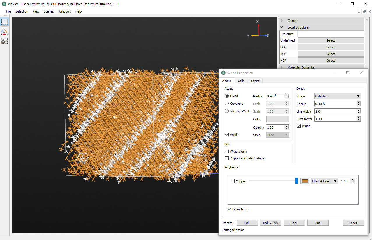
By rotating the cell, you will still see some grey regions, which are the remainders of the grain boundaries. The fast sliding and merging of the grains must be attributed to the small initial grain size, as this reduces the energy barrier upon changing their structure. The final structure appears locked by the periodic boundary conditions of the small cell, and little additional sliding to release energy is possible.
After the structural inspection you may want to have a look at the output
observables, starting with the stress in the z-direction. The stress curve has
been saved to the file CreepStress.png:
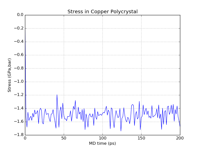
The graph shows that the stress oscillates at high frequency and stabilizes around the target value of -1.5 GPa. Generally, as long as the oscillations remain within reasonable bounds and do not increase in magnitude you don’t have to worry about this behavior.
The time-dependent creep strain is plotted in the file
CreepStrain.png. The curves denote the strain in the x (green) and z
(blue) directions, respectively:
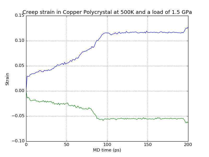
Although your example may look different from the results shown here (due to the random nature of the polycrystalline supercell building process) it should have some common features. In the beginning of the simulation a rapid increase of z-axis strain to about 2% is visible. This contribution arises from the immediate elastic deformation of the solid and it should be to a large extent reversible. Following that, a continuous – but much slower – increase in strain takes place. Here, the grain structure relaxes irreversibly by sliding and diffusion, or even structural transformation. Note that at around 90 ps a jump in the creep curve becomes visible, which must be attributed to a major (inelastic) structural rearrangement.
Important
Be aware that we are considering only the initial onset of creep behavior in a very small model system with very few grains and grain sizes in the order of less than one nanometer! The observed behavior might thus not be transferable in a straightforward way to real polycrystals with considerably larger grain sizes.
The elongation is accompanied by a transverse shrinking of the simulation box, as visualized by the x-strain, from which one can calculate the Poisson ratio of the polycrystal.
Finally, take a look at the time-dependent potential energy:
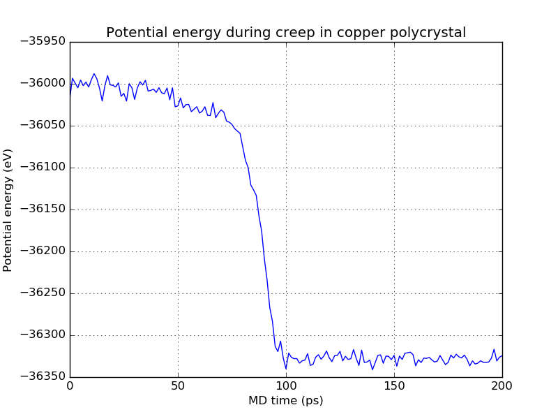
After the initial elastic deformation, which is of course accompanied by an increase of energy (it can be hard to see in the plot, it is very sudden), the creep process leads to a continuous decrease of potential energy caused by relaxation processes within the grain structure. As already observed in the creep strain, the same pronounced jump at 90 ps appears in the potential energy curve as well. From its magnitude, you can see that the corresponding relaxation process is accompanied by a large release of energy.
Outlook
Using the Polycrystal Builder, you can easily build huge polycrystal systems with a large number of grains. The following example shows a copper polycrystal of 300 x 300 x 300 Å3. The system contains around 2.3 million atoms.
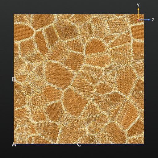
Simulations of such huge systems are perfectly possible with the ATK- Classical simulation engine, but will naturally take longer time, and one has to be careful with the size of the output files. The picture also nicely demonstrates the great graphical performance of QuantumATK – rotating and manipulating this crystal in 3D can be done completely fluently.