Open-circuit voltage profile of a Li-S battery: ReaxFF molecular dynamics
Version: 2017.1
Sulfur is a promising cathode material for rechargeable energy storage devices. During battery discharge, lithium ions migrate from the Li-rich anode to the sulfur cathode, and react with the sulfur (lithiation of the cathode):
The open-circuit voltage (OCV) is the electrochemical driving force for this lithiation process.
In this tutorial we apply molecular dynamics (MD) simulations to calculate the OCV profile during cell discharge. We use the ATK-ForceField calculator and employ the ReaxFF force field developed by Islam an co-workers in Ref. [1]. The simulated annealing method is used to simulate amorphous LixS compounds for a range of compositions \(x\), and the resulting OCV profile is compared to that in Fig. 3 in Ref. [1].
Note
Fig. 3 in Ref. [1] was made using data from a hybrid grand canonical Monte Carlo/molecular dynamics (GC-MC/MD) method, which is currently not available in QuantumATK. Instead of using the GC-MC to place Li atoms into low energy sites, we use here a simulated annealing method.
Theoretical definition of the open-circuit voltage
Neglecting enthalpic and entropic energy contributions, the OCV is calculated from total-energy differences:
where \(n\) (\(m\)) is the number of lithium (sulfur) atoms in the LixS compound (such that \(x=n/m\)), and \(E_\textrm{Li}\) and \(E_\textrm{S}\) are the total energies per atom of the pure Li and S crystals, respectively.
Outline
We first consider Li0.4S and describe all steps needed to compute the open-circuit voltage for partial lithiation of pure S to Li0.4S:
ATK Python scriting is then used for more automated simulations for a range of LixS compositions. The full OCV profile is computed and radial distribution functions for different compositions are investigated:
Tip
QuantumATK Python scripts are provided for download throughout this tutorial.
You may also download all of them in a single ZIP file: scripts.zip.
Note
This is an advanced tutorial – certain basics of operating the ATK-ForceField calculator and the QuantumATK analysis tools are not explained in great detail. Please see the tutorial How to Setup Basic Molecular Dynamics Simulations if needed.

Amorphous Li0.4S compound
The cahtode material is not expected to be in a perfect crystalline phase under battery operating conditions; it is most likely amorphous. QuantumATK offers several different tools for generating amorphous structures, for example the Amorhpous Prebuilder and the PackMol tool. We use here the latter.
Open QuantumATK and create a new project, preferably in a new directory on your harddrive.
The open the  Builder.
PackMol
The initial structure of the amorphous Li0.4S compound is here generated using PackMol, which randomly mixes input molecule configurations into a reasonable amorphous bulk configuration. You therefore need to first add atomic sulfur and atomic lithium to the Builder Stash:
In the Stash, click to add a hydrogen atom in a molecule configuration.
Select the H atom and use the
 tool to turn the H atom into S.
Repeat the two steps above to create also a lithium atom.
Rename the Stash items “sulfur” and “lithium”, respectively.

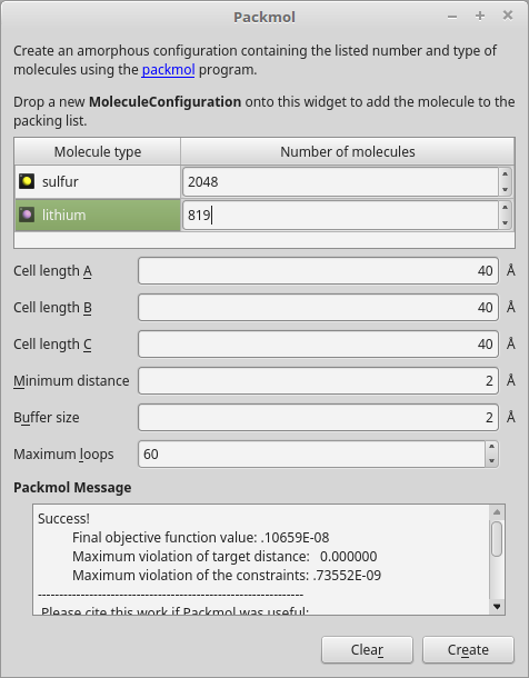
Navigate to the plugin and click it. The PackMol widget should now open. Do the following to create a Li0.4S amorphous crystal containing 2048 sulfur atoms.
Drag-and-drop the sulfur and lithium atoms from the Stash onto the PackMol widget. The configurations will be added to the “Molecule type” list.
Increase the number of sulfur entities to 2048, and the number of lithium entities to 819 (computed from 2048 \(\times\)0.4 = 819).
Leave all other settings at their defaults, and click Create.
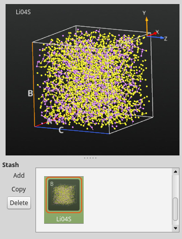
The amorphous Li0.4S structure is automatically added to the Stash. Rename it “Li04S”.
Geometry optimization
The amorphous structure produced by PackMol is guarenteed to have some minimal distance between all mixed entities (2 Å by default), but the structure may still be far from equilibrium. It is therefore a good idea to run an optimization of the atomic coordinates and lattice vectors before heating the system to a high temperature using MD.
Send the “Li04S” configuration to the
 Script Generator
and add the
Script Generator
and add the  New Calculator and
  OptimizeGeometry script blocks.
Open the calculator block, and select the ATK-ForceField calculator. The ReaxFF_LiS_2005 force field is automatically selected – it was generated in Ref. [1].
Open the geometry optimization block, and increase the force tolerance to 0.5 eV/Å and increase the maximum number of optimization steps to 1000. Also tick the Save trajectory option and enter
Li04Sas the file name for saving the relaxation trajectory.
Save the QuantumATK Python script as Li04S.py and run it using either
the  Job Manager or manually in a terminal:
atkpython Li04S.py 2>&1 | tee Li04S.log
You may also download the script: Li04S.py.
Important
Parallelizing ATK-ForceField calculations over more than one physical core is most efficiently done using OpenMP threading rather than MPI, see the relevant sections in tutorials on using the Job Manager for local and remote QuantumATK calculations with threading only.
If running QuantumATK from a terminal, the environment variable OMP_NUM_THREADS
should either be unset or set to the maximum number of OpenMP threads
you intend to use.
We recommend to set MKL_DYNAMIC=TRUE to allow MKL to dynamically
change the number of threads.
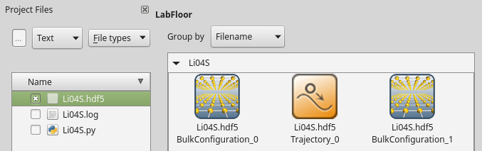
The geometry optimization should now have finished, and the output data should be available on the QuantumATK LabFloor:
You may use the  Viewer to visualize the relaxation trajectory;
you will see that the unit cell expands a bit upon minimization of atomic forces
and stress on the cell.
Viewer to visualize the relaxation trajectory;
you will see that the unit cell expands a bit upon minimization of atomic forces
and stress on the cell.
Simulated annealing
The room temperature structure of the amorphous Li0.4S compound (atomic coordinates and unit cell vectors) is not know a priori, so we use the simulated annealing method to find it. The basic idea is to heat up the system 1600 K and then slowly cool it down to 300 K using molecular dynamics, all at fixed pressure but allowing the unit cell volume to adapt (NPT dynamics).
The computational workflow is this:
Equilibrate the system at 1600 K.
Slowly cool down the system from 1600 to 300 K.
Equilibrate the system at 300 K.
Equilibration at 1600 K
The bulk configuration labeled BulkConfiguration_1 on the LabFloor
(saved in Li04S.hdf5) is the optimized one.
Select it and drop it on the Scripter.
The appropriate ATK-ForceField calculator block is automatically added,
so add just the MolecularDynamics script block.
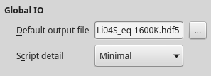
First, set the default output file name to Li04S_eq-1600K.hdf5:
Then open the MD script block and adjust the settings:
Select the NPT Berendsen MD type.
Increase the number of MD steps to 50000.
Increase the log interval to 1000.
Set the both reservoir temperature and the final temperature to 1600 K.
Set also the temperature for the Maxwell–Boltzmann distribution of initial particle velocities to 1600 K.
Optional: Untick the Save trajectory option.
Click OK to save te settings.

Save the script as Li04S_eq-1600K.py and run it. Depending on the
computational resources (number of OpenMP threads), the job may take up
to an hour to finish.
You may also download the QuantumATK Python script: Li04S_eq-1600K.py.
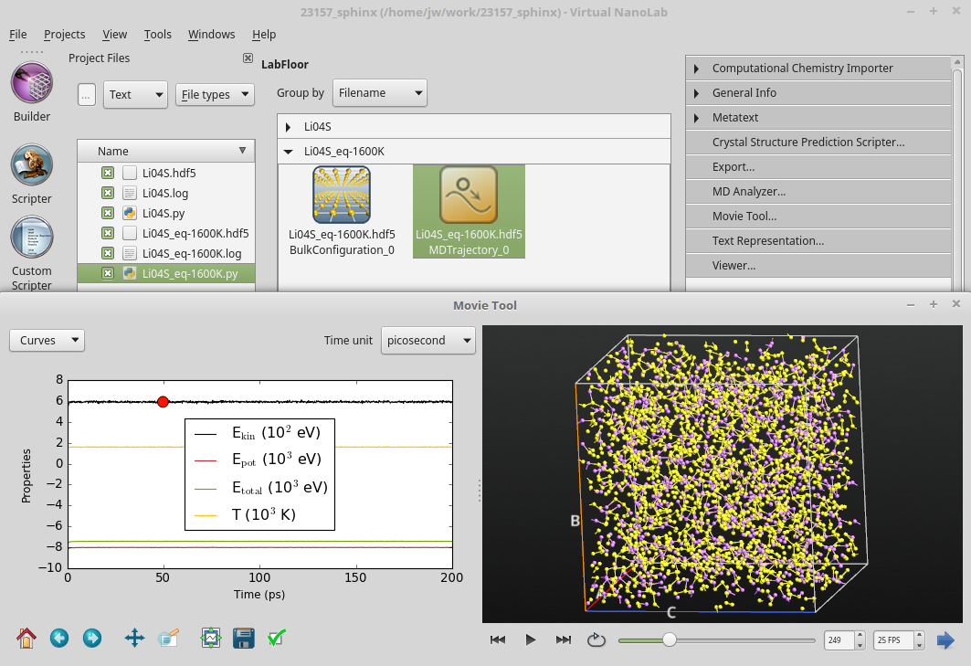
Once the calculation is done, the resulting MD trajectory should pop up on the LabFloor. Use the Movie Tool to visualize the progress of the MD simulation. You can use mouse right-click to enable the Show bonds option if needed. Note how the temperature and energies stay roughly constant throughout the simulation, and that the unit cell expands significantly at the beginning, but then stays fairly constant while the atoms move around inside it. The configuration is thereby equilibrated at constant temperature.
Cool-down from 1600 to 300 K
The Li0.4S configuration is now equilibrated and ready to be cooled down to room
temperature. In the Movie Tool, use the  icon to
transfer the last MD image in the MD trajectory to the
Scripter.
icon to
transfer the last MD image in the MD trajectory to the
Scripter.
Add the New Calculator and
MolecularDynamics script blocks,
and select again the ATK-ForceField calculator with the appropriate force field.
Then set the default output file name to Li04S_cool-down.hdf5,
and adjust the settings for the MD block:
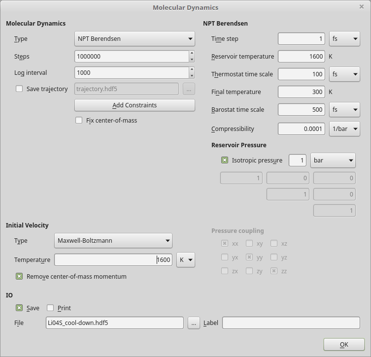
Select the NPT Berendsen MD type.
Increase the number of MD steps to 1 mio.
Increase the log interval to 1000.
Set the reservoir temperature to 1600 K and the final temperature to 300 K.
Set the temperature for the Maxwell–Boltzmann distribution of initial particle velocities to 1600 K.
Optional: Untick the Save trajectory option.
Click OK to save te settings.
This will result in a linear temperature ramp over 1 ns of MD simulation time (106 steps \(\times\)1 fs/step = 1 ns), and a cooling rate of 1.3 K/ps.
Save the script as Li04S_cool-down.py and run it.
You may also download the QuantumATK Python script: Li04S_cool-down.py.
Warning
The calculation may take a full day if executed on a single core, so it is recommended to use threading when running this job.
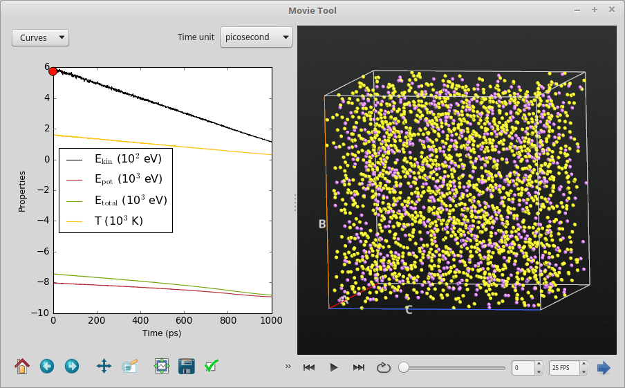
Once the calculation is done, the resulting MD trajectory should become available on the LabFloor. Use again the Movie Tool to visualize the progress of the MD simulation. Notice how the temperature decreases linearly from 1600 K to 300 K, and that the energies of the system decrease as well. Moreover, running the movie from start to end, it is clear that the Li0.4S unit cell shrinks when cooled down, quite as expected.
Equilibration at 300 K
Final step is to equilibrate the room temperature amorphous Li0.4S structure.
In the Movie Tool, use again the icon to transfer the last MD image
from the cool-down MD trajectory to the Scripter.
Add the New Calculator and
MolecularDynamics script blocks,
and select again the ATK-ForceField calculator with the appropriate force field.
Then set the default output file name to Li04S_eq-300K.hdf5
and adjust the settings for the MD block:
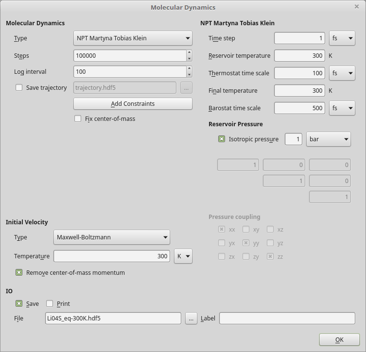
Select the NPT Martyna-Tobias-Klein MD type.
Increase the number of MD steps to 100000.
Increase the log interval to 100.
Set the reservoir temperature to 300 K.
Set the temperature for the Maxwell–Boltzmann distribution of initial particle velocities to 300 K.
Optional: Untick the Save trajectory option.
Click OK to save te settings.
Save the script as Li04S_eq-300K.py and run it.
You may also download the QuantumATK Python script: Li04S_eq-300K.py.
Once the calculation is done you may use the Movie Tool to check that the calculation went as expected (constant temperature, etc.).
The plot below shows the evolution of the total energy per atom and the
volume as the MD equilibration progresses. Both energy and volume reaches
a stable mean (the black dashed lines), and are thefore well equilibrated
after 1000 MD steps. The script evolution.py was used to generate the plots.
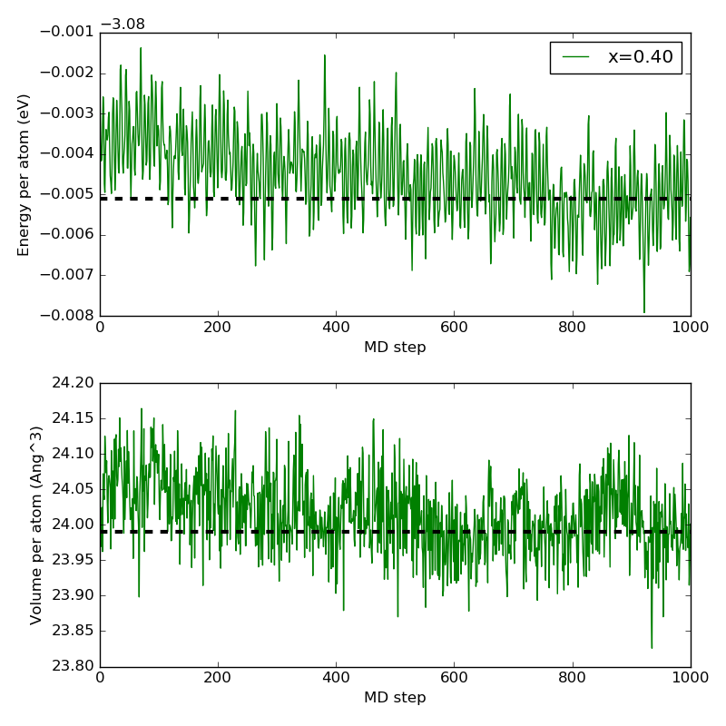
Fig. 80 Evolution of the total energy per atom (top) and the volume (bottom) as the MD equilibration progresses. Black dashed lines indicate the average over the last 100 MD images.
Open-circuit voltage
The OCV is calculated from total-energy differences as discussed in the introduction.
Each total energy should be for a geometry optimized structure.
To check that the calculated OCV does not depend significantly on the chosen
equilibration MD image, you should first perform geometry optimization at fixed
unit cell volume for several of the last equilibrated images, and compute the
corresponding OCV values. Use the script Li04S_relax.py to do this.
You also need the total energy per atom of the pure BCC Li and ORTH S8 crystals.
The scripts Lithium.py and a-Sulfur.py perform the required geometry optimizations
and calculate the total energies. Run both scripts.
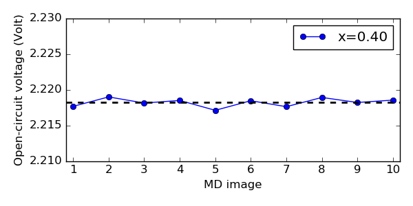
Then calculate and plot the OCV for all the 10 selected Li0.4S MD images
using the script ocv.py.
The plot is shown below. The black line indicates the average OCV, and it is clear
that even though choosing different MD images from the equilibration MD simulation
results in slightly different OCV values, they are very similar.
For each LixS composition, we shall below use the average OCV over 10 MD images.
Full open-circuit voltage profile
So far, we have obtained the OCV for Li0.4S. To plot the full OCV profile for litiation to the sulfur cathode corresponding to the reduction pathway of S8 to LixS, you should repeat the procedure outlined above for a range of Li concentrations. However, that may be a somewhat tedius workflow – some degree of automation would be useful.
ATK Python scripting is ideal for assembling the different
MD scripts given above for Li0.4S into a single script that will run all
calculations for a given lithium concentration.
The script x0.40_full.py does this for \(x\)=0.4.
Download it and use it as a template for running all required MD simulations
for each composition:
Use PackMol to generate structures for the desired compositions and save each structure in a separate data file named
x#.##.hdf5, where#.##indicates the Li concentration, e.g.0.40.Run a separate script for each LixS composition (copy
x0.40_full.pyand edit it to use the above generatedhdf5file as input and output data file.)
Note
Calculations for Li-rich compounds may take several days even if executed on 16 cores using OpenMP threading.
The cool-down MD simulation takes by far the largest part of the job wall-time. You may be able to decrease the time-to-result by decreasing the number of MD steps used in the cool-down from 1600 K to 300 K (and thereby increase the cooling rate), but be careful in doing so, since the cooling rate may affect your results.
Also, it turns out that equilibration often converges faster for Li-rich structures than for dilute Li concentrations, so it may be possible to decrease the number of MD steps for those simulations also.
Finally, plot the OCV profile over the LixS compositions using the script ocv_profile.py.
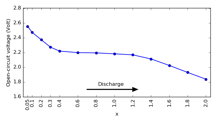
Fig. 81 Open circuit voltage profile during lithiation of the sulfur cathode.
This plot shows the full OCV profile and it is almost same as in Fig. 3 in [1]. Typically, experimental discharge voltage profiles for a Li-S battery can exhibit two or three reduction stages depending on the electrolyte. In this case, ReaxFF molecular dynamics calculations predict an initial drop, a flatter region, and again a voltage drop, all in agreement with experiments.
The initial drop may be induced by the formation of high-order polysulfides, i.e. sulfur-rich compounds from the S8 crystal. But it is not stable enough, so it is a fast process. The plateau at ~2.1 V is assigned to a slow process involving the further reduction to low-order polysulfides, i.e. Li-rich compounds. Here we only consider the litiated cathode, but in reality, these are very complex processes that may need more detailed understanding depending on the electrolyte composition.
Radial distribution functions
It is also useful to analyze the radial distribution functions (RDFs)
for S–S, Li–Li and S–Li in different LixS compositions.
You may use the following scripts to obtain the plots given below:
rdf_lili.py, rdf_ss.py and rdf_sli.py.


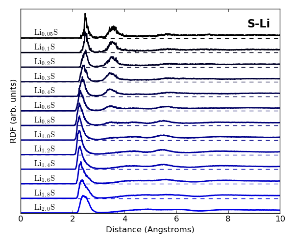
The RDFs for Li–Li, S–S and S–Li distances compare well with Fig. 5 in [1], and clearly indicate that 1) Li–Li bonds at ~3 Å distance are formed upon Li uptake during lithiation of the sulfur cathode, 2) short S–S bonds disppear upon Li uptake, and 3) both short and long S–Li distances exist for small Li contents, but the short S–Li bonds (~2.5 Å) dominate at large Li uptake.