Thermoelectric effects in a CNT with isotope doping

Although the mass of the nucleus has almost no influence on the electronic properties of an atom (at least in the Born-Oppenheimer approximation), different isotopes will have different thermal properties. The consequences of isotope doping are very important for the case of 1D nanostructures and nanotubes in particular [1], [2], [3]. It is therefore interesting to study how the thermal properties of a CNT change when the isotope distribution in one part of the tube is changed [4].

In this tutorial, you will study the effect of doping a carbon nanotube with a ring of ¹⁴C atoms. Specifically, you will calculate the phonon and electron transmission spectra, the thermal conductance, and the ZT product. You will use the ATK-ForceField engine for phonon calculations, while electronic transmission is calculated using ATK-SE.

Attention

This tutorial assumes that you have already finished the tutorial Simple carbon nanotube device, where the CNT device configuration used in this tutorial is created. If not, please go through that tutorial first, or simply download the configuration here: cnt_device.py.

CNT device with tags for ¹⁴C doping

Drag and drop the undoped CNT device configuration (cnt_device.py) onto the Builder . Then, assign a tag to the ¹²C atoms that you will convert to ¹⁴C:

• Select a ring of C atoms in the middle of the structure as shown below.

• Open the Selection Tools ‣ Tags plugin, and assign the tag “C14” to these atoms.

Phonon transmission

First set up and run the calculation of the phonon transmission spectrum for the undoped CNT. Transfer the configuration to the Script Generator and add the following blocks:

• New Calculator

• Analysis ‣ PhononTransmissionSpectrum

Note that a DynamicalMatrix object was automatically added as well. Change the output file to cnt_phonons.hdf5 and edit the settings in all three blocks:

• Calculator: Select the ATK-ForceField calculator and the “Tersoff_C_2010” potential.

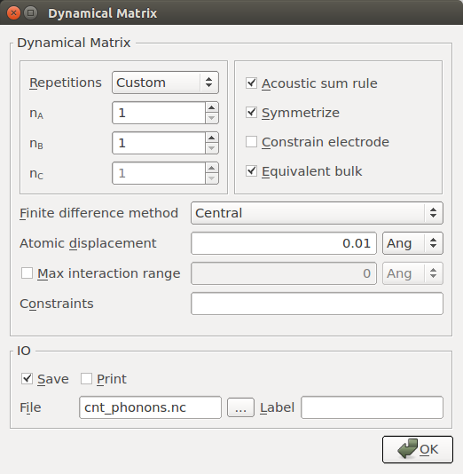
• DynamicalMatrix: Set “Repetition” to “Custom” and leave the repetitions along A, B, and C at the default value 1.

• PhononTransmissionSpectrum: Set the energy range to 0-0.3 eV and the number of points to 501. Leave the q-point sampling at defaults.

Note

For QuantumATK-versions older than 2017, the ATK-ForceField calculator can be found under the name ATK-Classical.

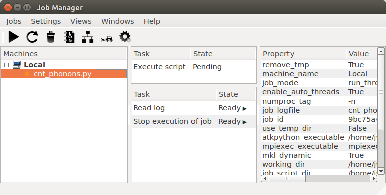
Run the calculation by sending it to the Job Manager . When prompted, save the script as cnt_phonons.py, select the default “Local” machine, and start the script by clicking .

Adding ¹⁴C impurity atoms

Once the calculation for the undoped CNT has finished, it is time to introduce the ¹⁴C dopants. The predefined elements in QuantumATK are isotope averages, so the mass of carbon in QuantumATK is 12.0107 amu. In order to create ¹⁴C, all you need to do is a bit of simple Python scripting: Implement a new element by writing a derived Python class with a different mass, and add it to the list of available elements. Do it like this:

• Open your Python script (cnt_phonons.py) in the Editor , e.g. using drag and drop.

• Find the place where the device_configuration is defined (lines 447-450). Insert the following lines of code immediately after:

  # Define a new class where the C atom has mass 14.00
  class C14(Carbon):
      @staticmethod
      def atomicMass():
          return 14.00*Units.atomic_mass_unit
  
  PeriodicTable.ALL_ELEMENTS.append(C14)
  
  # Replace all atoms tagged "C14" with carbon-14
  for index in device_configuration.indicesFromTags("C14"):
      device_configuration.elements()[index] = C14
  

• Change the output filename to cntc14_phonons.hdf5 everywhere in the script (3 places).

• Save the script as cntc14_phonons.py and execute it using the Job Manager.

Transmission spectra

The QuantumATK LabFloor should now contain the calculated results for the doped and undoped CNT:

• DynamicalMatrix

• PhononTransmissionSpectrum

Highlight the transmission spectra and use the Transmission Analyzer plugin to display the results. If you select both of them at the same time (holding down “Ctrl”), you can plot both in the same figure by using the Compare Data plugin.

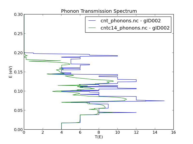
The two phonon transmission spectra in the above figure (blue: undoped CNT, green: isotope doped CNT) are significantly different. The difference is caused by phonon scattering by the ring of ¹⁴C impurities. You can see that at low energy (long wavelength) the spectrum is unchanged, while the main difference is at higher energies (shorter wavelength).

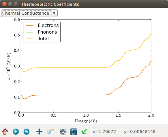
Thermal conductance

You can also calculate the thermal conductance of phonons, \(\kappa\)_ph, using the Thermoelectric Coefficients plugin, situated in the right-hand side of the LabFloor. Select again the PhononTransmissionSpectrum elements and click “calculate” on the Thermoelectric Coefficients plugin. As expected, \(\kappa\)_ph of the isotopically doped CNT is lower than for the CNT with a natural isotope distribution. The difference is small at 300 K, but it increases with temperature. The same effect was reported in [4], where the CNT was also doped by ¹⁴C, but in a cluster arrangement.

It is interesting to construct a plot similar to Figure 11(b) in [4]. You can do this by applying a bit of Python scripting. Save the Python code below as plot_thermal_conductance.py or simply download the script: plot_thermal_conductance.py. If you wish to understand how the script works, try to have a look at the entry about the PhononTransmissionSpectrum object in the PhononTransmissionSpectrum.

# Read the phonon transmission spectrum from file cnt_phonons.hdf5
phonon_transmission_spectrum = nlread("cnt_phonons.hdf5",PhononTransmissionSpectrum)[0]
# Define a temperature range
temp = numpy.linspace(10,2000,21)
# Calculate the phonon thermal conductance at each temperature 
conductances = []
for t in temp:
    conductance = phonon_transmission_spectrum.thermalConductance(
        phonon_temperature=[t]*Kelvin)
    conductance = conductance*10**9
    conductances.append(conductance)

# Now read the phonon transmission spectrum from file cntc14_phonons.hdf5 ...
phonon_transmission_spectrum_c14 = nlread("cntc14_phonons.hdf5",PhononTransmissionSpectrum)[0]
# ... and calculate the relative phonon thermal conductance
conductances_c14 = []
for t in temp:
    conductance_c14 = phonon_transmission_spectrum_c14.thermalConductance(
        phonon_temperature=[t]*Kelvin)
    conductance_c14 = conductance_c14*10**9
    conductances_c14.append(conductance_c14)

# Plot the phonon thermal conductances as function of temperature
import pylab
pylab.figure()
pylab.plot(temp,conductances,label='CNT',linewidth=2.0)
pylab.plot(temp,conductances_c14,label='14C-CNT',linewidth=2.0)
pylab.xlabel("Temperature (K)")
pylab.ylabel("Phonon Thermal Conductance (nW/K)")
pylab.legend(loc="lower right")
pylab.show()

Run the script in the directory where your .hdf5 files are stored:

$ atkpython plot_thermal_conductance.py

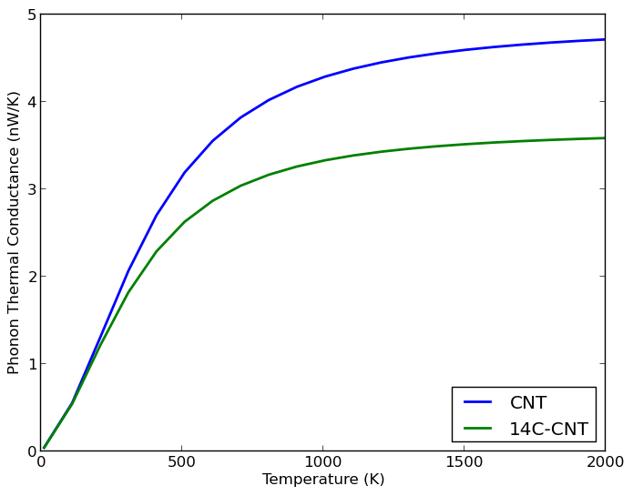
Fig. 85 Phonon thermal conductance of a pure CNT and of an ¹⁴C isotope doped CNT. The thermal conductance levels out with increasing temperature. The ¹⁴C doping clearly inhibits the CNT thermal conductance.

Electron transmission

The thermoelectric figure of merit, ZT, has both phononic and electronic contributions. Therefore, even though isotopic doping does not affect the electron transport properties, it is still relevant to calculate the electronic transmission spectrum for the CNT.

From the Builder send again your CNT device configuration to the Script Generator and add two blocks:

• New Calculator

• Analysis ‣ TransmissionSpectrum

Change the output file to cnt_electrons.hdf5 and edit the calculation parameters:

• Calculator: Select the ATK-SE: Slater-Koster calculator and choose the “Hancock.C ppPi” basis set.

• TransmissionSpectrum: Set the energy range to -10 to 10 eV and the number of points to 501.

Run the script using the Job Manager .

In the LabFloor you will now find the TransmissionSpectrum object, which you can plot using the 2D Plot plugin.

• TransmissionSpectrum

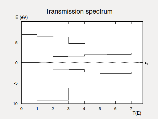
The electronic transmission is clearly non-zero in the vicinity of the Fermi level. However, if you zoom in, you will see that the transmission is zero exactly at the Fermi level. This is also clear if you study the transmission data using the Text Representation plugin.

Thermoelectric transport properties

Now you have all the ingredients for calculating thermoelectric transport properties such as conductance, Peltier coefficient, Seebeck coefficient, and heat transport coefficients of electrons and phonons, all of which are ingredients in the thermoelectric figure of merit, ZT.

Select from the LabFloor both the PhononTransmissionSpectrum AND the TransmissionSpectrum objects (by holding down “Ctrl” while clicking them). Open the Transmission Coefficient plugin and set the Fermi level shift to 0.04 eV, corresponding to the band edge. Finally, click Calculate to compute all the transport coefficients, and in particular the value of ZT at room temperature.

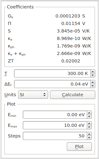
By clicking Plot, you can also get an interactive window with plots of the different transport quantities as a function og energy.

Compare ZT for doped and undoped CNTs

If you compare the two values of ZT for the two devices with and without ¹⁴C doping, you will find that the effect of isotopic doping is to slightly increase ZT. The effect is indeed very small.

One way to illustrate this result is by plotting ZT as a function of the energy for both CNTs in one figure. Once again, a bit of Python scripting will do the job. Use the following piece of Python code, or simply download the script: plot_zt.py.

from AddOns.TransportCoefficients.Utilities import evaluateMoments
from NL.CommonConcepts import PhysicalQuantity as Units

# Set input parameters
e_min = 0.0
e_max = 2.0
n_steps = 400
temperature = 300.00*Kelvin
energies = numpy.linspace(e_min, e_max, n_steps) * eV

# Read phonon transmission spectrum from file cnt_phonons.nc
# and get the phonon conductance at the specified temperature
phonon_transmission_spectrum = nlread('cnt_phonons.nc', PhononTransmissionSpectrum)[0]
conductance_phonons = phonon_transmission_spectrum.thermalConductance(phonon_temperature=temperature)

# Read phonon transmission spectrum from file cntc14_phonons.nc
# and get the phonon conductance at the specified temperature
phonon_transmission_spectrum_c14 = nlread('cntc14_phonons.nc', PhononTransmissionSpectrum)[0]
conductance_phonons_c14 = phonon_transmission_spectrum_c14.thermalConductance(phonon_temperature=temperature)

# Read electron transmission spectrum from file cnt_electrons.nc
electron_transmission_spectrum = nlread("cnt_electrons.nc",TransmissionSpectrum)[0]

# define lists for ZT data
zzt = []
zzt_c14 = []

# Calculate the ZTs at each energy
for energy in energies:
    # Calculate moments of the electron transmission spectrum
    k0, k1, k2 = evaluateMoments(electron_transmission_spectrum, temperature, energy)
    # Calculate transport properties.
    conductance       = k0*Units.e**2
    peltier           = k1/(k0*Units.e)
    seebeck           = k1/(k0*Units.e*temperature)
    thermal_electrons = (k2*k0-k1*k1)/(temperature*k0)
    total_thermal     = thermal_electrons + conductance_phonons
    total_thermal_c14 = thermal_electrons + conductance_phonons_c14
    zt                = conductance*seebeck**2*temperature/total_thermal
    zt_c14            = conductance*seebeck**2*temperature/total_thermal_c14
    zzt.append(zt)
    zzt_c14.append(zt_c14)

# Plot the ZT as function of energy
zzt = numpy.asarray(zzt)*1e3
zzt_c14 = numpy.asarray(zzt_c14)*1e3
import pylab
pylab.plot(energies,zzt,'-',label='CNT',linewidth=1.0,color='b')
pylab.plot(energies,zzt_c14,'--',label='14C-CNT',linewidth=1.0,color='r')
pylab.xlabel('Energy (eV)')
pylab.ylabel('ZT x 1000')
pylab.legend(loc='upper center')
pylab.show()

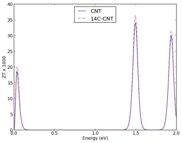
Fig. 86 ZT at 300 K for a CNT with a natural isotopic distribution (blue line) and for a CNT with a full ring of ¹⁴C impurities (red broken line).

The script produces the figure shown above. It is clear that isotopic doping increases the value of ZT, though only marginably.

References

[1]

Yong-qiang Cheng, Shu-yun Zhou, and Bang-fen Zhu. Isotope effect on phonon spectra in single-walled carbon nanotubes. Phys. Rev. B, 72:035410, Jul 2005. doi:10.1103/PhysRevB.72.035410.

[2]

Gang Zhang and Baowen Li. Thermal conductivity of nanotubes revisited: Effects of chirality, isotope impurity, tube length, and temperature. The Journal of Chemical Physics, 2005. doi:10.1063/1.2036967.

[3]

C. W. Chang, A. M. Fennimore, A. Afanasiev, D. Okawa, T. Ikuno, H. Garcia, Deyu Li, A. Majumdar, and A. Zettl. Isotope Effect on the Thermal Conductivity of Boron Nitride Nanotubes. Phys. Rev. Lett., 97:085901, Aug 2006. doi:10.1103/PhysRevLett.97.085901.

[4] (1,2,3)

Jin-Wu Jiang, Jian-Sheng Wang, and Baowen Li. A nonequilibrium Green’s function study of thermoelectric properties in single-walled carbon nanotubes. Journal of Applied Physics, 2011. doi:10.1063/1.3531573.