Inelastic Electron Spectroscopy of an H2 molecule placed between 1D Au chains
Version: 2017
This tutorial is focused on simulating inelastic electron tunneling spectroscopy (IETS) [1] for a device consisting of two one-dimensional (1D) gold electrodes and an H2 molecule placed in between. After DFT calculations of the dynamical matrix and the Hamiltonian derivatives with respect to vibrations of the H2 molecule, IETS is computed and analyzed based on the lowest-order expansion (LOE) [2] and extended LOE (XLOE) [3] approximations.
Note
It is assumed that you are familiar with QuantumATK. If not, go through the basic QuantumATK Tutorials first.

Introduction
We consider electron transport through a device consisting of an H2 molecule clamped between 1D gold electrodes. In a spectroscopy experiment, if the applied bias is comparable to the energy of one of the vibrational modes of the H2 molecule, a new inelastic transmission channel opens in which the transmission of electrons is mediated by the emission of a phonon. The coupling process is due to the coupling between electronic and vibrational degrees of freedom, that is, to the electron-phonon coupling. At a voltage where an inelastic channel opens, the derivative of the conductance, i.e., the second-derivative of the current has a peak. In experiments, IETS is defined by
and is measured to investigate, e.g., the electron-phonon coupling strength, heating, configuration, and local doping.
In the tutorial, you will first compute the dynamical matrix and the Hamiltonian derivatives with respect to vibrations of the H2 molecule by DFT calculations, and then calculate and analyze the IETS signal based on two different approximations: LOE and XLOE. The rest of this tutorial is hence organized as follows:
Device setup,
Calculation of the dynamical matrix and the Hamiltonian derivatives,
Calculation of IETS based on LOE and XLOE,
Analysis of IETS based on the vibrational modes of the H2 molecule,
Comparison between the LOE and XLOE results.
Device setup
Start up QuantumATK and create a new project. Instead of using  Builder to create the device configuration, we use the QuantumATK Python script
 au-h2-au_0.py, which provides the Au|H2|Au device. Download and save the script in the project folder, and open it from  Script Generator.
Add a
 New Calculator block and select GGA as the exchange correlation functional in the setting.
Note
The k-point sampling is by default 1x1x93, which should, however, be modified properly if the device is periodic in the A and/or B directions.
Set the output-file name “au-h2-au.nc”, and save the python script as “au-h2-au.py”.
Note
The python script must now be the same as au-h2-au.py. To save time, one may just download the script and use it.
Send the script to
 Job Manager and run it.
Calculation of IETS
The IETS calculation requires information of the dynamical matrix, which is defined in terms of the force for displacing the hydrogen atoms back and forth in each spatial direction. The computation involves six DFT calculations, which are all independent with each other, and is hence performed efficiently by using six CPU cores.
In the
Script Generator, click on  from File and select “au-h2-au.nc”.
Add a
 object and set it as follows:

Add also a
object and keep the default settings.
The IETS calculation requires information of the Hamiltonian derivatives as well. This calculation also consists of six independent parts, and is hence carried out efficiently using six CPU cores.
Add a
block and set it as follows:

Add an
, choose LOE as the method, and set the rest as follows:

Add another
block, and set it in the same way except choosing XLOE as the method.Set the output-file name “analysis.nc”, and save the python script as “analysis.py”.
Note
The python script must be the same as analysis.py. To save time, one may just download the script and use it.
Send the script to
Job Manager and run it.
The calculation will take less than one hour if six CPU cores are used, and save every result in “analysis.nc”.
Note
See InelasticTransmissionSpectrum in QuantumATK Manual, which provides a brief description about IETS and how it is computed from the dynamical matrix and the Hamiltonian derivatives. See also, e.g., Ref. [2] for more details.
Analysis
Vibrational modes of the H2 molecule
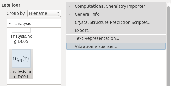
In the Labfloor, look at the vibrational modes of the H2 molecule by selecting the  Vibrational Mode object in the “analysis.nc” file with the help of Vibration Visualizer plugin.
There are, in total, six modes: Four transverse modes 0, 1, 2, 3; two longitudinal modes 4 and 5. The two pairs of modes (0 and 1) and (2 and 3) are, respectively, doubly degenerated. Note that the temperature is set T = 1000 K in the movies below to see the vibrations clearly.

Mode 0: 25.44 meV; Mode 1: 25.63 meV (the small energy difference is due to numerical error)
Mode 2: 60.54 meV; Mode 3: 60.56 meV (the small energy difference is due to numerical error)

Mode 4: 127.46 meV

Mode 5: 264.06 meV
IETS
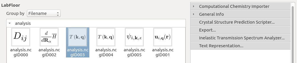
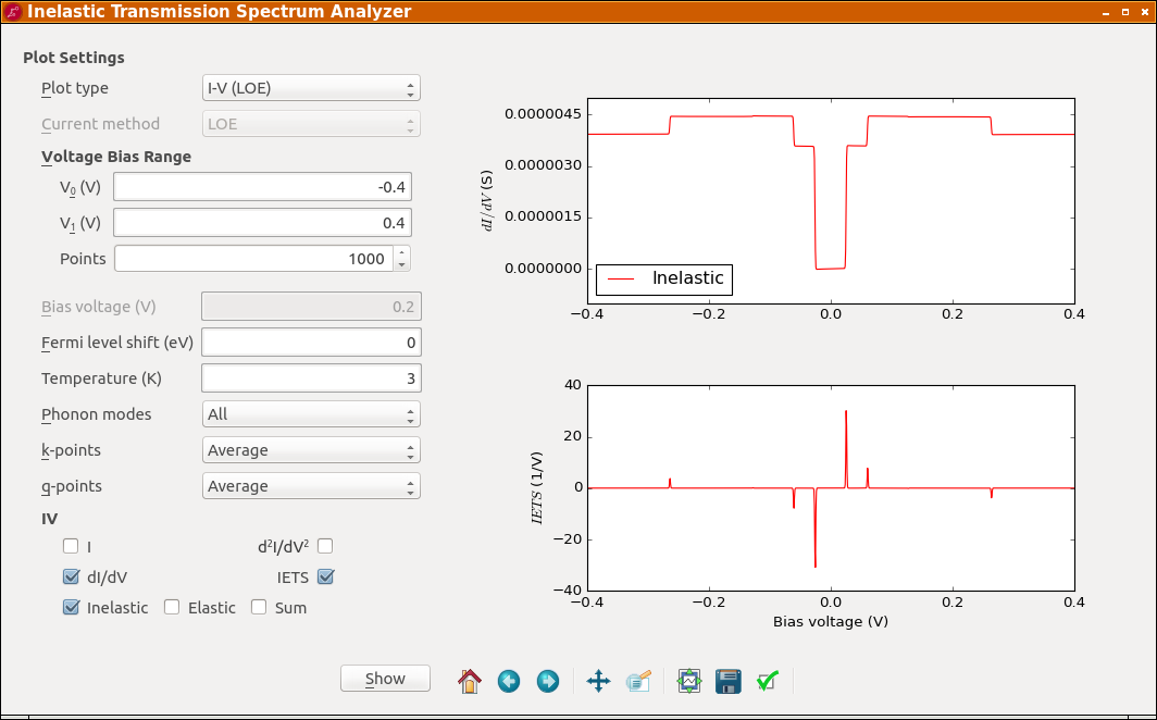
Then look at IETS. Select one of the  InelasticTransmissionSpectrum objects \(T({\bf k},{\bf q})\) in LabFloor and click on the Inelastic Transmission Spectrum Analyzer plugin, a new plugin available from ATK2017.
Set the panel as follows and click Show.
Attention
Because the density of states (DOS) of the gold electrodes is almost flat within this bias window, there only exists a minor difference between the LOE and XLOE results. See the discussion below for more details.
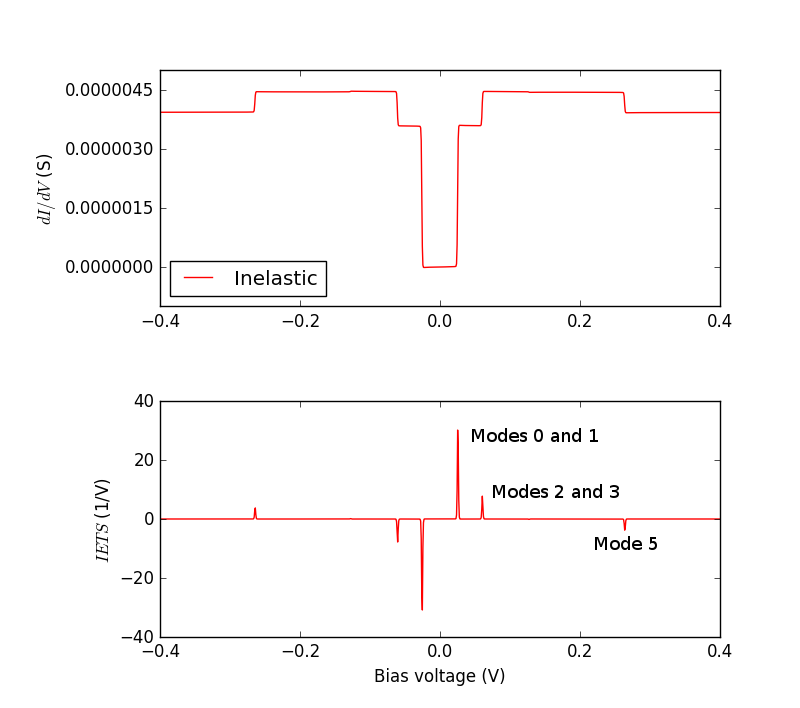
There appear three significant inelastic features (steps in conductance and peaks in IETS). Note that the inelastic conductance is increased by the coupling to the low-frequency transverse modes 0-3 and decreased by the coupling to the high-frequency longitudinal mode 5. Analyzing the scattering states clarifies the reason of the increases.
Drag the
 TransmissionEigenstates object \(\psi_{i,{\bf k},\epsilon}\) in LabFloor into
  Viewer. Then drag the
  DeviceConfiguration into Viewer.
Go to properties and, under the Isosurface flag, set the Isovalue to 0.5.

The scattering eigenstate has a clear d-symmetry on the gold chain. Hence, it couples only very weakly to the s-like states of the hydrogen atoms. The elastic transmission is thus small. The coupling to the transverse modes 0-3 can, however, open new inelastic channels and leads to positive steps in conductance and steps in IETS.
Detailed analysis of transmission: Comparison between LOE and XLOE
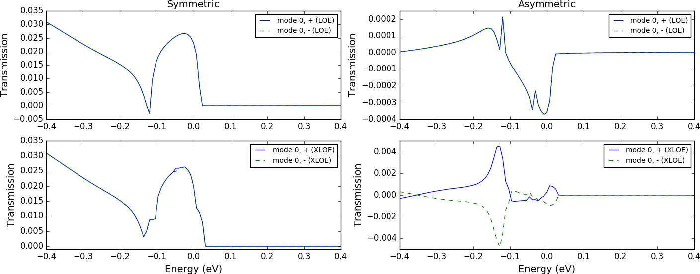
In the same window of the Inelastic Transmission Spectrum Analyzer plugin, now choose Transmissions in Plot type, set the options as shown below, and click Show. In this case, one will look at the positive symmetric and asymmetric parts of the inelastic transmission:

To understand some details of the transmission, note that, in either LOE or XLOE, the current as a function of the bias voltage \(V\) and the temperature \(T\) reads
where \(\epsilon_F\) is the Fermi energy, and the rest of the new symbols are defined as follows: In either approximation, the universal functions appear in the same form,
where \(G_0=2e^2/h\) is the conductance quantum, \(n_F(\cdot)\) is the Fermi-Dirac distribution function, and \(\mathcal{H}_{\epsilon'}[\cdot](\epsilon)\) means the Hilbert transform. In XLOE, the transmission functions are given by
with
and
This XLOE expression of the transmission functions reduces to the LOE expression by setting \(\mu_L=\mu_R=\epsilon\). Importantly, in the expression of the current, note that the Green’s function, the self-energies, and the spectral functions in the transmission functions are evaluated at two different energies \(\epsilon_F\pm \hbar\omega_{\lambda}\) in XLOE, whereas they are all evaluated at the same energy \(\epsilon_F\) in LOE. See Ref. [3] for more details.
For direct comparison between the LOE and XLOE results, see here below the inelastic transmissions for each phonon mode. The lines of positive/negative (a)symmetric transmissions indicate the plots of \(\mathcal{T}^{(a)sym}_{\lambda}(\epsilon)\) as functions \(\epsilon\) with setting \(\mu_R=\epsilon\pm \hbar\omega_{\lambda}\). The positive and negative (a)symmetric parts are exactly the same in LOE by definition, but different in XLOE.
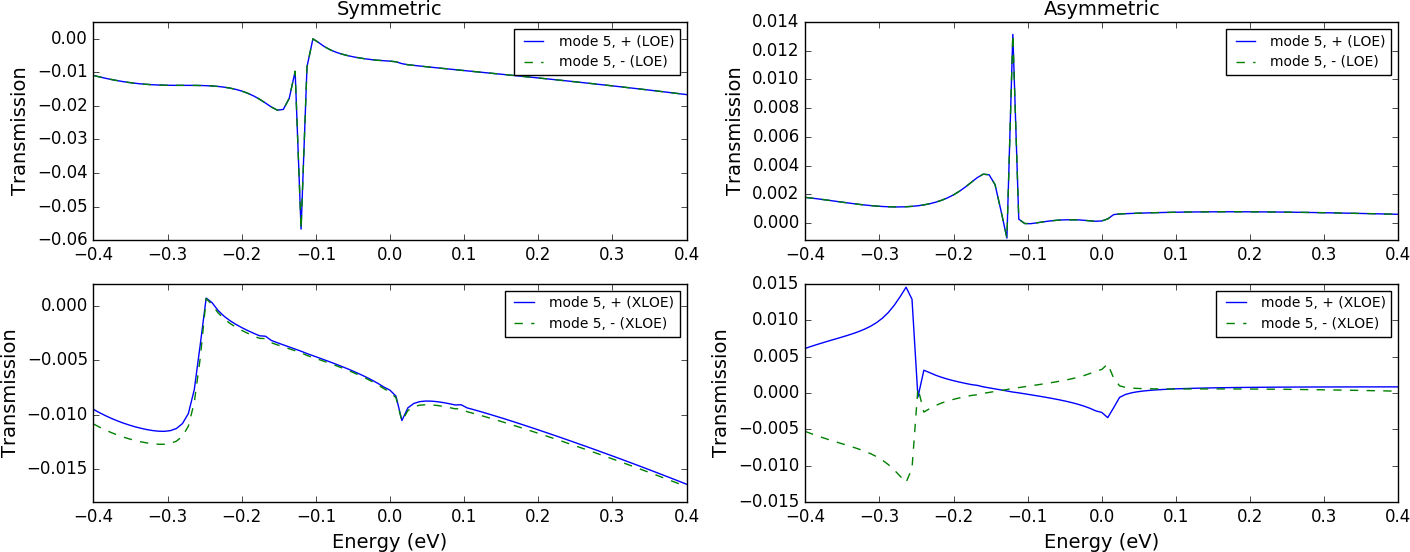
The LOE and XLOE results are in good agreement in areas where the transmission varies slowly as a function of \(\epsilon\). Around -0.11 eV, however, the wide-band approximation in LOE, i.e., the approximation \(\mu_L=\mu_R=\epsilon\), breaks down due to the presence of a resonance in the DOS of the 1D gold chain. As a result, there appears a difference between the LOE and XLOE results. The symmetric and asymmetric inelastic transmissions for mode 5 show the difference very clearly. The single peak at -0.11 eV in LOE splits into two peaks in XLOE; the separation is about 264 meV, which corresponds to the phonon energy of mode 5.