Stone–Wales Defects in Nanotubes
A Stone–Wales defect changes the connectivity of two \(\pi\)-bonded carbon atoms by rotating them 90° with respect to the midpoint of their bond, as illustrated below:
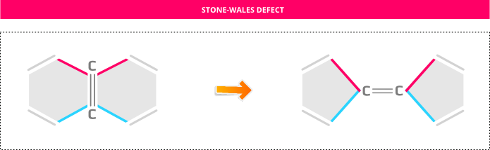
It is a crystallographic defect that occurs in e.g. nanotubes and graphene, and can have a strong influence on the electronic, chemical, and mechanical properties. It is named after Anthony Stone and David Wales of Cambridge University, who described it in a 1986 paper on fullerenes [1], but a similar defect was described much earlier by Peter Thrower in a paper on defects in graphite [2].
Note
You will create the Stone–Wales defect in graphene and then wrap it into a tube.
You will therefore need the TubeWrapper addon. Download the TubeWrapper.zip file and install the addon following the instructions in the AddOns page.
Creating the defect and wrapping the tube
Step 1: First create a graphene sheet by using the plugin. Select n=9 and m=0 for the chiral indices, and click Build.

Step 2: The purpose is to study an isolated defect, so it is necessary to make a large structure where a single carbon–carbon bond can be rotated. Repeat the configuration 10 times along the C direction using the tool, and press Ctrl+R to reset the view.

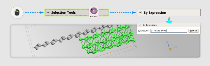
Step 3: Next, create the defect: Select two atoms in the middle of the structure, and open the tool. Select the rotation axis to be X (this is the default) and enter 90 degrees for the rotation angle. It is important that the checkbox Rotate around selection center is ticked. Then click Apply.

Step 4: You can now wrap the graphene sheet into a tube. The sheet is periodic along the B and C directions. The tube axis should be along C, so the graphene sheet should be rolled up along B. Use the tool to accomplish this; set the angle to 360 degrees and click Apply.
Optimizing the structure
The defect was created by a simple rotation of two carbon atoms, and is most likely not in its equilibrium shape. You should therefore geometry optimize the defect. The ATK-ForceField engine with the Brenner potential will provide a great starting point (conveniently available in ), but for a truly correct structure, you should run a full DFT optimization. In both cases, the ends of the tube should be constrained so they remain perfectly periodic, in order to use it for a device calculation later on.
Anyway, as a first approximation, select the defect atoms (white and pink in the figure below), and atoms immediately around the defect, to locally optimize the defect geometry. Use the Quick Optimizer with the Brenner potential (you will need to increase the number of steps to 100).

Then, convert the structure to a device using (just click Create, the default settings are fine).

Save the device in a file (say) as Device_stone.hdf5 in your project directory for other future calculations.
Transmission spectrum
Let’s extract the transmission spectrum of the last device structure. This is a rather large device – the central region contains 360 atoms – but with the ATK-SE engine you can calculate the electron transmission spectrum in just a few minutes.
Use the Script Generator to create a Python script including a Slater–Koster calculator with the Hancock.C ppPi basis set and a TransmissionSpectrum analysis block. Then run the calculation using the Job Manager, and use the 2D Plot plugin to visualize the calculated transmission spectrum.
The resulting transmission spectrum is also available for download:
Device_stone.hdf5.
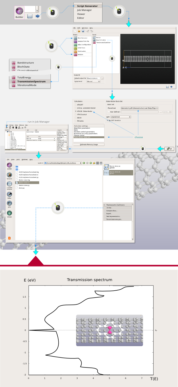
The transmission spectrum is shown above. It was computed using the Hancock single-band tight-binding model with up to 3rd nearest neighbor interactions from Ref. [3]. A perfect (9,0) tube would have a step-like transmission spectrum around the Fermi level, but the defect introduces strong scattering and significantly modifies the electronic transmission. This will most certainly have a noticeable influence on the I-V curve.
Tip
You can easily calculate the corresponding I-V curve: Simply start a new Script Generator session and use Analysis from File and the IVCurve analysis object to create the script. Plot the results using the IV-Plot plugin.
You can also calculate the transmission spectrum and I-V curve for the defect free (9,0) nanotube and compare to the results found above.