Transmission spectrum of a spin-polarized atomic chain
Version: 2016.3
In this tutorial, you will learn how to build an atomic-chain device, and calculate the spin-polarized transmission spectrum for two cases where the electrodes have parallel and anti-parallel spin-polarizations.
You will use a chain of carbon atoms to make the calculations run fast. Carbon is not naturally magnetic, but when the atom spacing in the chain is large enough – but not too large – the electronic ground state is actually spin-polarized. This system is of course highly artificial, and only chosen for the purpose of illustrating the methodology.

Building the 1D carbon chain
Open the QuantumATK
 Builder.
In the Stash, click . This creates a hydrogen atom.
Select the hydrogen atom in the 3D view and use the
 Periodic Table tool to convert the atom to carbon.
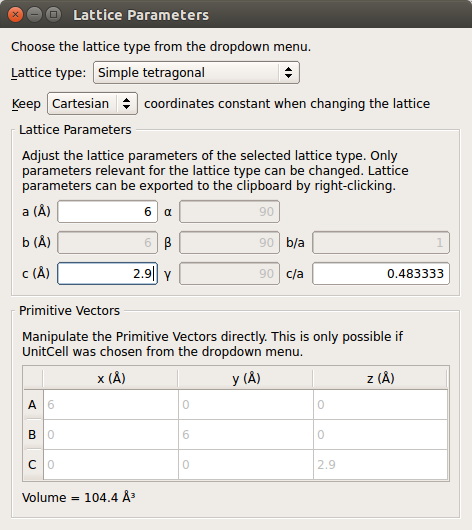
Open the tool and change the lattice type to Simple tetragonal. Then set the lattice constants to a = 6 Å and c = 2.9 Å.
Tip
Periodic boundary conditions will be employed along the A and B directions, so we use the large a = 6 Å unit cell vector to minimize electrostatic interactions between repeated images of the chain along A and B.
Click to center the atom in the unit cell.
Use the plugin to repeat the system 12 times in the C direction.
Use the plugin to create the carbon-chain device. The automatically suggested electrode length of 8.7 Å is adequate, so just click OK.

Spin-parallel transmission spectrum
You will now set up a NEGF-DFT calculation with parallel spins throughout the device, and compute the electronic transmission spectrum for this spin configuration.
Send the device configuration to the
 Script Generator
by using the Send to icon
Script Generator
by using the Send to icon  in the lower-right corner of the Builder.
Set the Default output file to
carbon_para.nc.Add a
 New Calculator block to the script, and
double-click it to open it.
New Calculator block to the script, and
double-click it to open it.Set the Spin to Polarized. The exchange–correlation functional will automatically switch to LSDA.

Add an
 Initial State block, which defines
the initial spin populations. Open it and select User spin
(all atoms now start out at maximum spin-up polarization).
Initial State block, which defines
the initial spin populations. Open it and select User spin
(all atoms now start out at maximum spin-up polarization).Add a
 block.
Default parameters are fine for this 1D carbon chain.
block.
Default parameters are fine for this 1D carbon chain.

The QuantumATK Python script is now ready. Send it to the
 Job Manager, save the script as
 carbon_para.py, and run the calculation – it should only take a few minutes to run.
Note
Do not close the Script Generator window – you will need it later on.
Tip
By inspecting the QuantumATK log file, note that the populations for the up/down (DM[U]/DM[D]) electronic states are nearly the same on all atoms, as expected in an ideal system. The small differences are primarily due to the fairly low default density mesh cut-off.
Analysis
The calculated TransmissionSpectrum analysis object should now be available on the QuantumATK LabFloor.
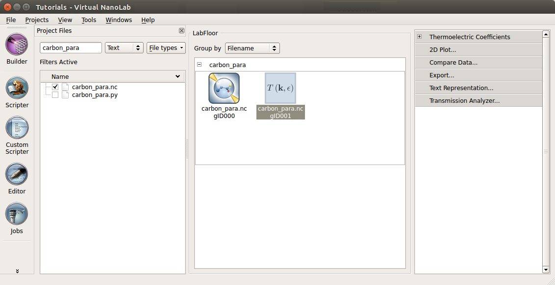
Select the TransmissionSpectrum and use the Transmission Analyzer to plot the spin-parallel transmission spectrum.

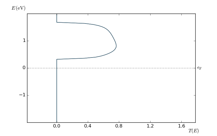
Both the up (light blue) and down (dark blue) spin components of the transmission spectrum are plotted, and they are significantly different: The spin-down transmission is zero at the Fermi level, where the (unitless) spin-up transmission is 3.
Spin anti-parallel transmission spectrum
You will now do the spin anti-parallel calculation and compare the transmission spectrum to that of the spin-parallel case. The already computed spin-parallel ground state will be used as an initial guess for the anti-parallel calculation.
Return to the Script Generator window and modify the
settings:
Change the Default output file to
carbon_anti.nc.Double-click the
InitialState block and modify
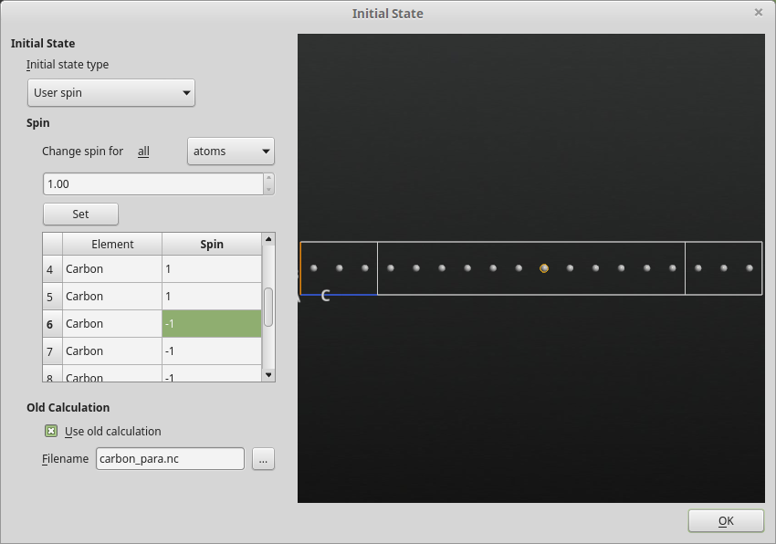
the following parameters:Set the initial state type to User spin
Set the spin on atoms with index 6 to 11 to -1.
Tick Use old calculation and set the Filename, from where to read the spin-parallel ground state, to
carbon_para.nc.
That’s it! Save the script as
carbon_anti.pyand run it using the Job Manager.
Analysis
When the calculation finishes, use again the Transmission Analyzer
to plot the transmission spectrum contained in carbon_anti.nc.
The two spin components have, in this case, identical transmission spectra,
as expected from the symmetry of the device.
Tip
If you inspect the QuantumATK log file from the anti-parallel calculation, you will see that the spin is indeed flipped in the right part of the device, where the spin-down density matrices, DM[D], have higher occupations than the spin-up ones, DM[U]:
+------------------------------------------------------------------------------+
| Density Matrix Report                         DM[U]     DM[D]      DD        |
+------------------------------------------------------------------------------+
|   0   C   [   3.000 ,   3.000 ,   1.450 ]    2.99639   1.00028  -0.00333     |
|   1   C   [   3.000 ,   3.000 ,   4.350 ]    3.00324   0.99997   0.00321     |
|   2   C   [   3.000 ,   3.000 ,   7.250 ]    2.99536   1.00105  -0.00359     |
|   3   C   [   3.000 ,   3.000 ,  10.150 ]    3.00271   1.00275   0.00546     |
|   4   C   [   3.000 ,   3.000 ,  13.050 ]    2.96897   1.01659  -0.01444     |
|   5   C   [   3.000 ,   3.000 ,  15.950 ]    2.92841   1.08262   0.01103     |
|   6   C   [   3.000 ,   3.000 ,  18.850 ]    1.08262   2.92840   0.01101     |
|   7   C   [   3.000 ,   3.000 ,  21.750 ]    1.01660   2.96897  -0.01444     |
|   8   C   [   3.000 ,   3.000 ,  24.650 ]    1.00275   3.00271   0.00546     |
|   9   C   [   3.000 ,   3.000 ,  27.550 ]    1.00105   2.99535  -0.00359     |
|  10   C   [   3.000 ,   3.000 ,  30.450 ]    0.99997   3.00325   0.00322     |
|  11   C   [   3.000 ,   3.000 ,  33.350 ]    1.00027   2.99629  -0.00344     |
+------------------------------------------------------------------------------+
Regarding the use of the spin-parallel calculation as initial state, QuantumATK will actually flip the density matrix if the initial spin (which is set in the InitialState block) is less than zero. Also, the spins in both electrodes are automatically set to match the spin configuration in the corresponding electrode extensions.
Finally, mark both the parallel and anti-parallel transmission spectra on the LabFloor, and use the Compare Data plugin to directly compare the total transmission in both cases. The transmission in the spin-parallel state (blue) is significantly larger than that of the anti-parallel state (green) over most of the sampled energy window around the Fermi level.
