Li-ion diffusion in LiFePO4 for battery applications
Version: 2016.3
LiFePO4 is among the typical rechargeable Li-ion battery cathode materials with high energy density and low cost, while also being environmentally friendly [1][2]. In this tutorial you will use ATK-DFT to estimate the Li-ion diffusion rates along different crystallographic directions in LiFePO4.
In particular, you will:
Import the LiFePO4 bulk structure.
Optimize the LiFePO4 lattice parameters.
Create the Li\(_{1-x}\)FePO4 structures.
Optimize the initial and final configurations.
Create initial NEB trajectories (IDPP interpolation).
Optimize the Li diffusion path.
Calculate the reaction rates using harmonic transition state theory (HTST).
Import LiFePO4 bulk structure
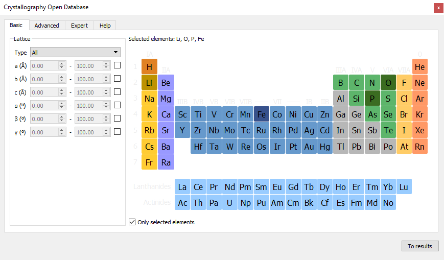
The LiFePO4 structure can be imported from the Crystallography Open Database plugin in QuantumATK.
Click the
 Builder.
Open the .
Select Li, Fe, P, O as elements and click the To results button.
Choose Lithium Iron Phosphate(V), Simple Orthorhombic(Pnma).
Click Add to stash button.
It will be automatically loaded in the Builder stash.

New functionality in QuantumATK 2017:
From the QuantumATK 2017 version, crystal structures such as LiFePO4 can be imported by the QuantumATK Databases tool as follows: Click the  DataBases. See COD (Crystallography Open Database) and Materials Project. Both are possible to get the LiFePO4 structure. In the COD case, select Li, Fe, P, O as elements and click the Search button.
You can also use the Materials Project database. Choose the Materials Project. Select elements or type LiFePO4. Select one and click the import button, it will be automatically loaded in the LabFloor in the same way as the COD. In this case, you can get more calculation information including the structure from the Material Project database.

For more options, see also Import XYZ, CIF, CAR, VASP files in QuantumATK tutorial.
Optimize LiFePO4 lattice parameters
You can import the LiFePO4 structure to the Builder to have a deeper look into the structure.
Note
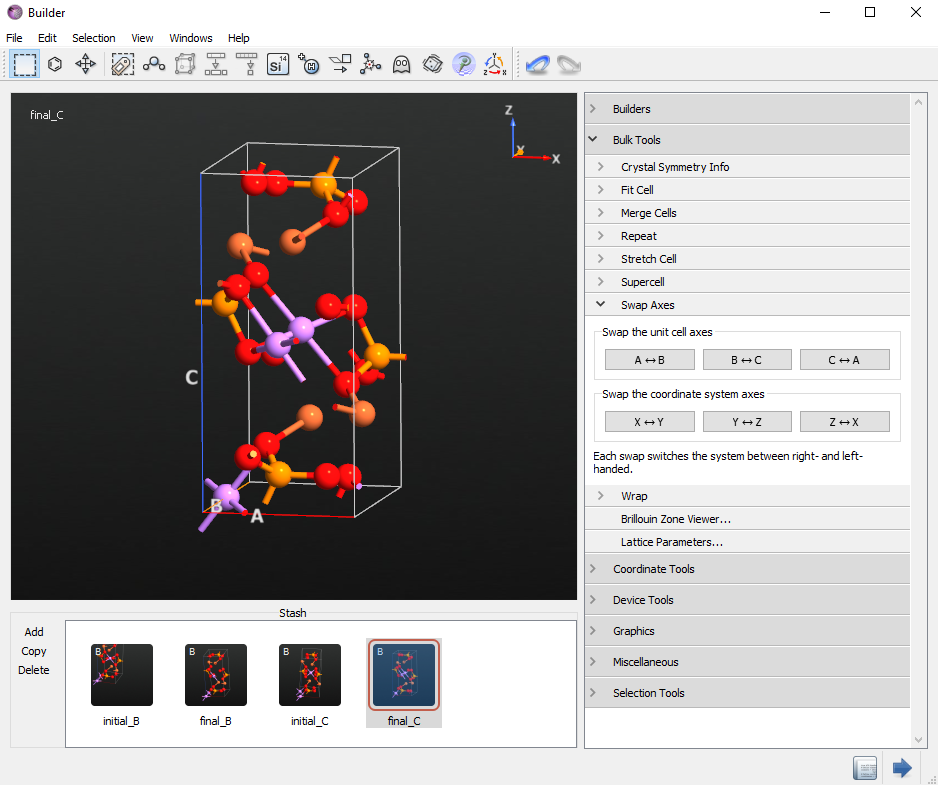
In order to better compare with the results of reference [3] you can use the tool to swap C<->A and Z<->X. However, by doing so, the configuration will lose the information about the symmetry type, in this case Simple orthorhombic. Use the tool to set the Lattice type to Simple orthorhombic.
In order to optimize the lattice parameters, send the LiFePO4 structure from the Stash to the Scripter to set up a new DFT calculation as follows:
Add the
 New Calculator block and modify the following parameters:
SGGA-PBE exchange correlation potential
7x5x3 k-point sampling
(We will use the the default FHI pseudopotentials and DZP basis set).
Add an
 OptimizeGeometry block and modify:
Max forces 0.02 eV/Å
Max stress 0.1 GPa
Remove check from Constrain cell to allow for cell optimization
Check Save trajectory and specify the file
LiFePo4_opt.nc
Change default output file name to
LiFePo4_opt.ncFinally, send the script to the JobManager and run the calculation.
It takes about 30 minutes on 8 cores. After finishing the job, open the optimized BulkConfiguration with object ID glD002 with the Builder.
Check the new optimized lattice parameters which agree to within 0.1 percent with the experimental data.
Create the Li\(_{1-x}\)FePO4 structures
In this tutorial you will study the diffusion of one Li atom for a Li-deficient structure such as Li\(_{1-x}\)FePO4. In particular, you will remove one of the four Li atoms from the bulk configuration. Note that the diffusion energy barriers depend on the Li concentration [4].
In the next section you will set up the calculation for the diffusion of a Li atom along two different directions. You thus need to create initial configurations and final configurations for the same Li atom diffusing along the B and C directions.
Create initial and final structures for diffusion along B direction
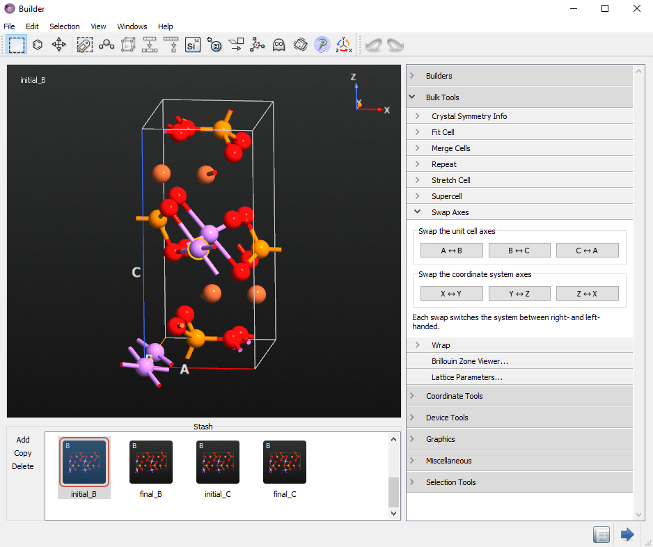
Right-click on the configuration on the Stash and make three copies such that you have 4 identical configurations. We will make initial and final structures for the B and C directions.
From the first configuration, delete one Li atom as in the figure below. This will be your initial structure for the B direction NEB calculations and you can rename it initial_B.
Double click the second configuration to make it active. Next rename it final_B. Select the same Li atom you just deleted from the initial configuration and open the
 Periodic Table tool. Click on Gold (Au) element to change the Li atom to Gold.
Tip
You are applying this trick to be able to move the Li atom into a specific position. In this case, the position of the Li vacancy defined by the Gold atom. There are indeed several other workarounds to build this final configuration, e.g. by copying the coordinates of the original Li atom you removed. You are welcome to use here the procedure that you find more relevant and intuitive for you.
Select Li atom number 7 (the one next to the Gold atom along the B direction) and use the
 Move tool to move it on top of the Gold atom. Be sure that the Snap option is enabled.
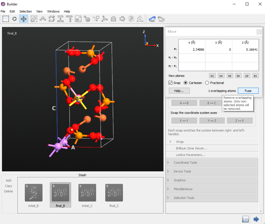
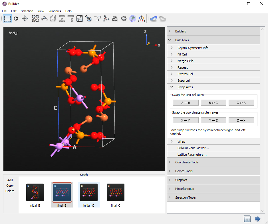
Use the Fuse option to remove the Gold atom and your final structure is now ready.
Finally, check the Li atom number 6 in the initial_B and final_B configurations. Li atom number 6 should be moved in the B direction.
Create initial and final structures for diffusion along C direction
Follow the same procedure as above to create the configuration along the C direction. The initial structure for the C direction is the same as the intial_B structure. Rename it initial_C. In this case, the final structure moves Li atom number 4 to the removed Li position (substituted Gold) in the inital_C structure. Rename the final structure, final_C.

Optimize initial and final configurations
Send each structure, initial_B, final_B, initial_C and final_C, to the Scripter and set up a geometry optimization calculation with the same parameters as for the LiFePO4 structure. However, in this case you will not optimize the lattice parameters. Check the Constrain cell option as indicated below.

Moreover, in this case you can use the unpolarized GGA.PBE functional. This will allow you to run your calculation much faster.
Here you can download the four input scripts: initial_B.py, final_B.py, initial_C.py and final_C.py.
Create initial NEB trajectories
The tutorial Pt diffusion on Pt surfaces using NEB calculations will teach you how to set up the NEB object. Here we will highlight only the main steps.
When the optimization of the end points are done you will find the optimized configurations loaded in the LabFloor with object ID equal to glD002. Drag and drop these BulkConfiguration objects directly into the Builder.
In the Builder open the plugin and drag and drop from the Stash the initial and final configurations corresponding to the diffusion of a Li atom along the B direction,
initial_B.ncandfinal_B.ncconfigurations.
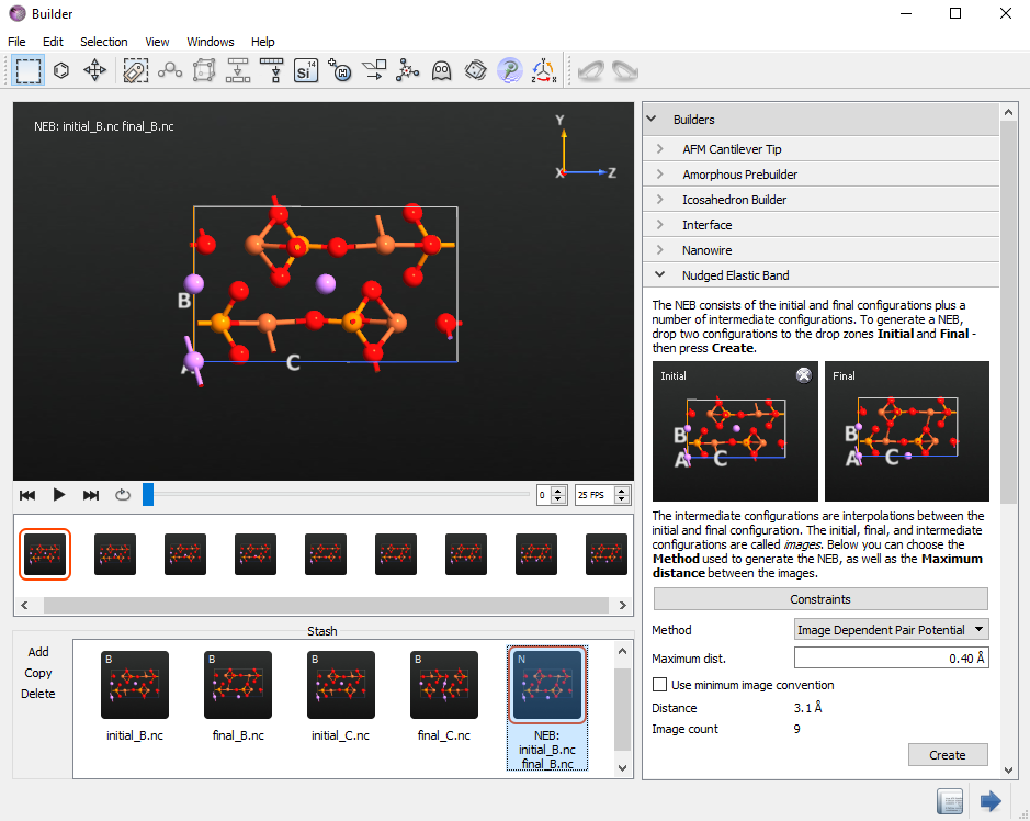
Select the Image Dependent Pair Potential interpolation method and use 9 images including the end points.
Create the initial Li diffusion path along C direction with the
initial_C.ncandfinal_C.ncconfigurations. Use 9 images with 0.8 Å maximum distance including the end points .
Optimize Li diffusion path
You are now ready to set up and optimize the Li diffusion path in LiFePO4.
Send the two NEB objects from the Stash to the Scripter.
Add and set up a
New Calculator with the same settings as for the calculators of the end points.Add a
OptimizeGeometry block and be sure to
select the Climbing Image Method.Finally, run the two NEB calculations
neb_B.pyandneb_C.py.
Note that as described in the Pt diffusion on Pt surfaces using NEB calculations, you can run this calculation in parallel over many MPI processes. In particular, a NEB run is parallelized over the internal images. ATK will try to detect the best parallelization strategy and it will write a small report at the beginning of your log file.
In this example, you will immediately see that a load balance problem has been detected. However, 2 out 16 cores will be idle, so it is a rather small loss of efficiency, not “greatly reduced” as it says in the log file below. It takes about 2 hours in 16 processes. You can also change the number of MPI processes you are using to achieve the best performance.
+------------------------------------------------------------------------------+
| NEB image level parallelism enabled.                                         |
+------------------------------------------------------------------------------+
| Total number of interior images: 7                                           |
| Total number of processes: 16                                                |
| Processes per image: 2                                                       |
| Images calculated in parallel: 8                                             |
|                                                                              |
| Process group # 0 will calculate images: 1                                   |
| Process group # 1 will calculate images: 2                                   |
| Process group # 2 will calculate images: 3                                   |
| Process group # 3 will calculate images: 4                                   |
| Process group # 4 will calculate images: 5                                   |
| Process group # 5 will calculate images: 6                                   |
| Process group # 6 will calculate images: 7                                   |
| Process group # 7 will be idle!                                              |
| WARNING: Load balance problem detected.                                      |
|          The number of interior images calculated in parallel is not a       |
|          divisor of the number of interior images. This will greatly         |
|          reduce parallel performance. Either modify the parameter            |
|          "processes_per_image" or the number of MPI processes.               |
|                                                                              |
|          With 2 processes_per_image ideal performance will be obtained       |
|          by using 14 MPI processes.
Tip
You can speed up the optimization by first running a simple NEB calculation with a high force tolerance, e.g. 0.08 eV/Å, and without using the Climbing Image Method. This will in general be a faster calculation giving you a rough estimate of the energy barrier and the diffusion path. After this step, you can set up a more precise NEB run and also use the climbing method to finalize your results.
Analyze the results
Once the calculation is properly converged you will find the optimized NudgedElasticBand object loaded in the LabFloor
Tip
Always remember to check the log file at the end of your simulation. In particular, check that convergence is achieved:
+------------------------------------------------------------------------------+
| NEB Optimization using the LBFGS optimizer                                   |
+------------------------------------------------------------------------------+
| Iteration   Step Length    Max. Force  Max. Energy Image    Max. Energy      |
+------------------------------------------------------------------------------+
|         0     0.000e+00     1.473e+00                  4       0.925917      |
|         1     4.825e-02     1.362e+00                  4       0.794101      |
...
|        23     1.220e-02     2.772e-01                  4       0.405770      |
|        24     3.731e-03     4.938e-02                  4       0.404796      |
+------------------------------------------------------------------------------+
| NEB optimization converged after 24 steps.                                   |
+------------------------------------------------------------------------------+
In the two figures below, the optimized Li diffusion process for the Li atom moving along the B and C directions are illustrated by using the Movie Tool plugin.

While the Li atom can more easily move along the B direction with 0.39 eV energy barrier, you found a high energy barrier, 2.3 eV for the Li atom moving along the C direction. The results are in agreement with reference [4].
Calculate the reaction rates using harmonic transition state theory
For detailed information about how reaction rates are calculated and the theory behind the harmonic transition state theory please refer to the Calculating reaction rates using harmonic transition state theory.
To set up the analysis:
Open the Scripter.
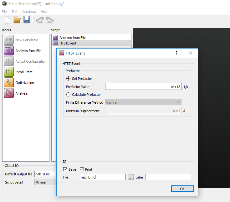
Double click on Analysis from file and select the
neb_B.ncconfiguration with object ID glD001.Add the HTSTEvent analysis and set the prefactor to 1e+13 1/s.
Run the analysis which will only take a minute. Here is the input script.
HTST_analysis.py
Note
The time required for an HTSTEvent analysis strongly depends on whether or not the prefactor is assumed or calculated. If you need to calculate the prefactor, it can take a long time, depending on the method and system. Therefore, it is usually a very good approximation to assume the prefactor for solid state reactions like bulk diffusion.
In order to visualize the results from the HTSTEvents analysis, select the corresponding object from the LabFloor and select the HTST Rates plugin on the right hand side.
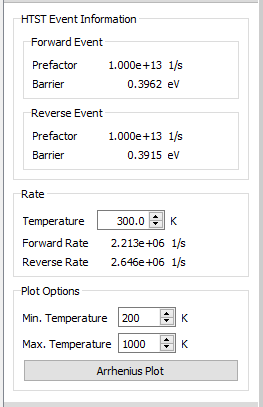
Here, you can calculate the forward and reverse reaction rates for your diffusion mechanism. In this case you will find these two values to be very close to each other because the initial and final states are essentially equivalent.
Here, you can also set the options for an Arrhenius plot:

The table below summarized the results found in this tutorial.
Direction |
Barrier |
k\(_{HTST}\) |
B |
0.39 |
2.6 x 10⁶ |
C |
2.30 |
1.9 x 10⁻²⁶ |