Poisson solvers
The Hartree potential
The self-consistent solution of DFT: LCAO, DFT: Plane Wave and Semi Empirical calculators requires the evaluation of the Hartree potential obtained from a given charge density via the solution of the Poisson equation:
Note that the Hartree potential has units of energy and represent the potential energy of an electron in the corresponding electrostatic potential.
The Poisson equation is a second-order differential equation and a boundary condition (BC) is required in order to fix the solution. The charge density which enters the Poisson equation is evaluate differently in Semi-Empirical and DFT methods (see The Hartree potential and the electrostatic potential and references therein). However, the Poisson equation and the BCs formulation are general and valid both for Semi-Empirical and DFT calculators.
In the following sections an overview of the boundary conditions and Poisson solvers available in QuantumATK is provided.
Boundary conditions
A simulated configuration is enclosed in a bounding box, and the Hartree potential is defined on a regular grid within this box. At the facets of the bounding box four basic types of BC can be applied: multipole, periodic, Dirichlet and Neumann.
The following BCs can be imposed on the six facets of the simulation box, with some limitations for specific solvers or configurations which will be listed in the following sections.
PeriodicBoundaryCondition BCs enforce periodicity of the solution along opposite facets.
MultipoleBoundaryCondition BCs are determined by calculating the monopole, dipole and quadrupole moments of the charge distribution inside the simulation cell, and that these moments are used to extrapolate the value of the potential at the boundary. They can be used to simulate charged molecules or system with a large dipole moment which would otherwise require a very large simulation box to allow the potential to go asymptotically to zero.
DirichletBoundaryCondition BCs constrain the potential on the exterior boundary points of a facet \(S\) such that:
\[V^{H}({\bf r}) = V_{0}({\bf r}), {\bf r} \in S\]\(V_{0}\) is set to 0 for all configurations except for the electrode facets in a SurfaceConfiguration or a DeviceConfiguration (see Boundary Conditions in NEGF).
In the vacuum facet of a SurfaceConfiguration an arbitrary value can be assigned.
NeumannBoundaryCondition BCs set a constraint on the normal derivative of the potential on a facet:
\[{\bf n} \cdot {\bf \nabla} V^{H}({\bf r}) = V^\prime_{0}({\bf r}), {\bf r} \in S\]Also in this case \(V^\prime_{0}({\bf r})=0\), but it is possible to specify a given value for the electric field on the vacuum side of a SurfaceConfiguration. For the electrode facets in a SurfaceConfiguration or a DeviceConfiguration the value of the derivative is calculate from the electrode bulk potential (see Boundary Conditions in NEGF).
The BCs are imposed by using the keyword boundary_conditions, supported by any
Poisson solver:
poisson_solver = MultigridSolver(
boundary_conditions=[[PeriodicBoundaryCondition(),  PeriodicBoundaryCondition()],
                        [DirichletBoundaryCondition(), DirichletBoundaryCondition()],
                        [PeriodicBoundaryCondition(),  PeriodicBoundaryCondition()]]
)
Note
Periodic or Neumann boundary conditions only determine the Hartree potential up to an additive constant, which reflects the physics that the bulk electrostatic potential does not have a fixed value relative to the vacuum level. In this case the potential is internally shifted such that its average is zero.
Boundary Conditions in NEGF
When running NEGF calculations (i.e., DeviceConfiguration or a SurfaceConfiguration), the BCs at the facets where the electrodes are defined are treated in a special way.
Dirichlet BCs on the left surface of the simulation grid at equilibrium are set as:
where \(V_{bulk,left}(\mathbf{r})\) is the electrode bulk Hartree potential, \(V_{applied, left}\) the voltage applied on the left contact, \(e\) is the electron charge, and \(\Omega_{left}\) the left boundary surface. The electode bulk Hartree potential is pre-calculated at the beginning of a NEGF calculation.
On the right surface (for devices) we have:
where \(-|e|V_{built-in}=\mu_{bulk,right}-\mu_{bulk,left}\) is the built-in potential due to the difference of chemical potential in the isolated electrodes at equilibrium. This ensures continuity of the potential between the central region and the electrode at the boundary.
Neumann BCs can also be specified in the transport direction. In this case the derivative of the potential on the facet used as constraint is calculated on each point from the electrode bulk potential:
In doing so we enforce continuity of the potential in the central region and in the electrode, apart from a floating rigid shift.
For surfaces, where only the left electrode is defined, a constant value Neumann BC can be applied on the right facet of the grid (vacuum region).
Additional information about NEGF calculations can be found in NEGF: Device Calculators.
Dielectric and metallic regions
A user can define regions within the simulation box to simulate dielectric regions or metallic regions. This feature is typically used to simulate gated devices. For a metallic region \(\Omega\) the Hartree potential is fixed to a constrained value \(V_{0}\) within this region:
For a dielectric region \(\Omega\) with a given relative dielectric constant \(\epsilon_{r}\), the right hand side of the Poisson equation is modified as:
Moreover, QuantumATK allows to specify a relative dielectric constant to be used in the whole simulation box around the atoms to model an implicit solvent.
Poisson solvers
The following Poisson solvers are supported by QuantumATK:
FastFourierSolver uses a Fourier Transform with Periodic boundary conditions in all directions. This is a very fast method and the default when simulating BulkConfiguration with any calculator.
FastFourier2DSolver can be utilized to simulate DeviceConfiguration with Device calculator. It uses a Fourier transform in the directions perpendicular to the transport direction, and a real space multigrid method in the transport direction. It does not support metallic or dielectric region. However, it is fast and accurate and therefore it is the default method for devices without metallic and dielectric regions.
MultigridSolver uses a real space multigrid method. It allows for any kind of boundary conditions in all directions and supports metallic and dielectric regions. It is the default solver for devices with metallic and dielectric regions. It is an iterative method, therefore it is slighlty less accurate than the FastFourier2DSolver. It requires a moderate amount of memory, however it is not parallelized and it can be significantly slower than ParallelConjugateGradientSolver and NonuniformGridConjugateGradientSolver on a parallel environment.
ParallelConjugateGradientSolver uses an iterative solver based on the conjugate gradient method. Similar to the MultigridSolver, ìt allows for different types of boundary conditions, implicit solvents, and the use of metallic and dielectric spatial regions to simulate gates. This method is similar to MultigridSolver in terms of accuracy and outperforms it when running calculations in parallel. The solver utilizes PETSc [1] as backengine and it is parallelized.
NonuniformGridConjugateGradientSolver is an efficient method for BulkConfiguration and DeviceConfiguration with a large vacuum in the A and B directions, and as such is particularly suitable for the simulations of low-dimensional systems (i.e. nanowires, nanotubes, 2D materials). It evaluates the Poisson equation on an auxiliary non-uniform grid in order to reduce the number of degree of freedoms in the vacuum regions, and it is significantly faster and less memory consuming than other solvers in such cases. The solver utilizes the conjugate gradient solver from PETSc [1] as backengine and it is parallelized.
DirectSolver uses a direct real space solver method. It supports all different types of boundary conditions, implicit solvent, and the use of metallic and dielectric spatial regions. It requires significantly more memory than the other solver methods and it is slower than the Multigrid and the iterative solvers, but it is exact and can be used as a robust reference for small systems. The solver utilizes MUMPS [2] as backengine and it is parallelized.
Note
A tight convergence criteria is set internally for all iterative solvers. Sometimes the iterative solver might fail to converge and a warning is displayed, with an indication of the reached tolerance where applicable. If the error is small and the selfconsistent loop reaches convergence, the calculation is likely converged to a valid solution.
In the figure below support for the various BCs, spatial regions and implicit solvent for the different Poisson solvers is summarized.
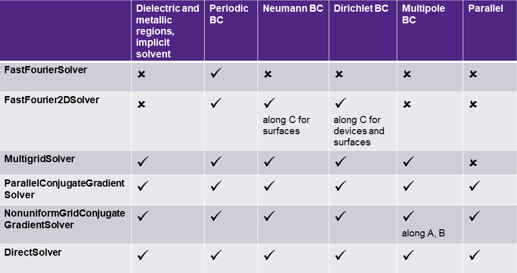
Fig. 213 Support for different BCs, dielectric/metallic regions and MPI parallelization for the available Poisson solvers.
In figures below a benchmark on a Silicon slab is shown, where
all available solvers are compared. The structure is repeated in the A, B direction 1, 2 or 3 times
to vary system size. The calculation parameters are chosen such that the runtime is dominated
by the calculation of the Hartree potential and a single selfconsistent step is performed.
The reported time considers only the time spent assembling and solving the Poisson equation,
while the memory is the total system peak memory.
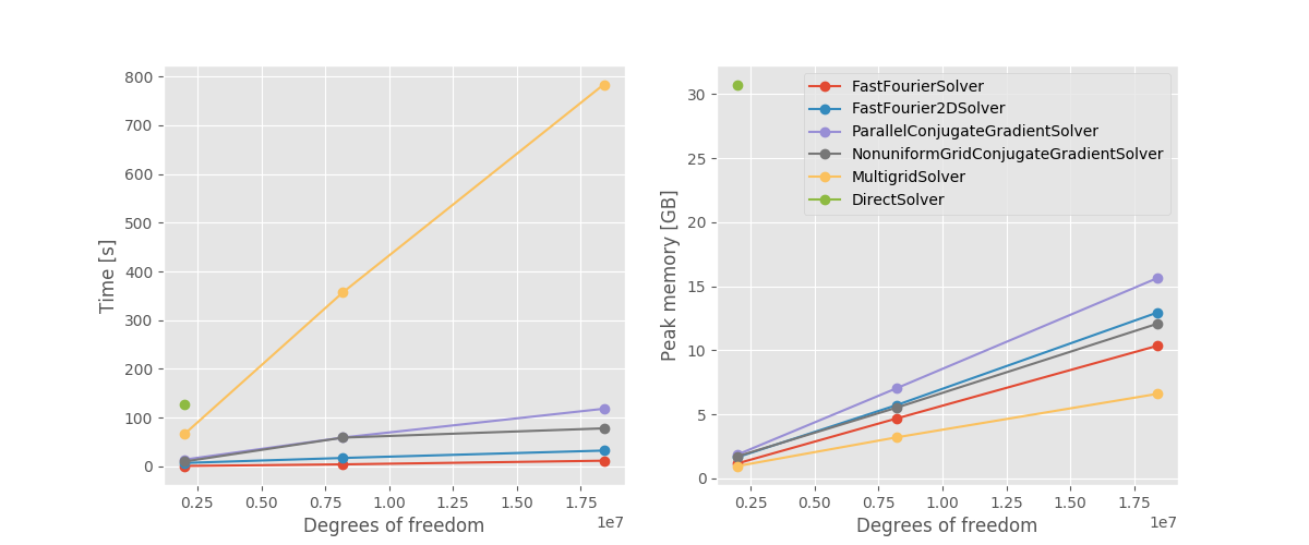
Fig. 214 Wallclok time and peak memory consumption as a function of the system size, expressed as number of degrees of freedom of the real-space grid. All calculations are performed on a single Intel(R) Xeon(R) CPU E5-2650 node using 8 MPI processes. For the DirectSolver only one data point could be computed, due to memory limitation.
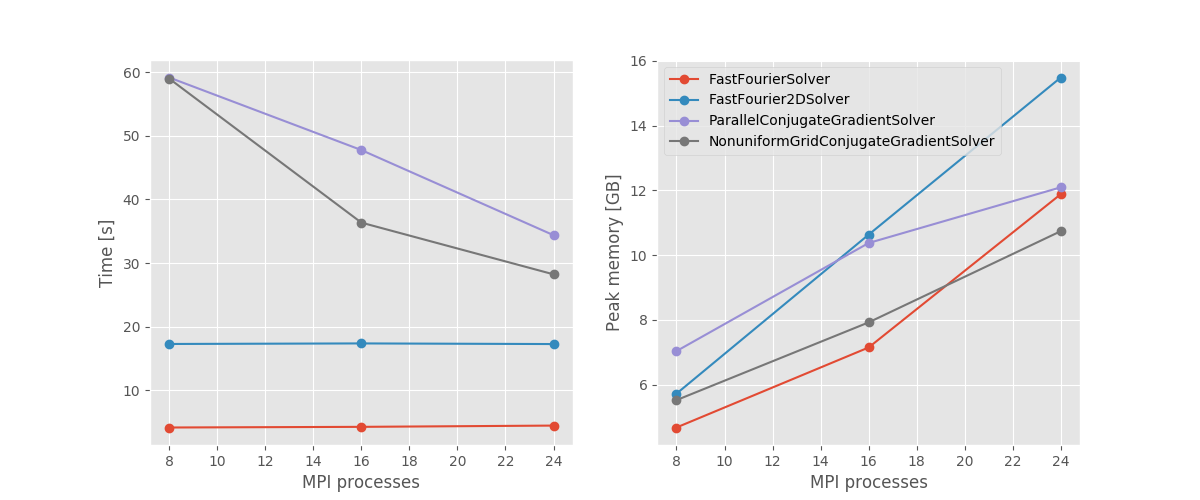
Fig. 215 Wallclok time and peak memory consumption as a function of MPI processes. All calculations are performed on a single Intel(R) Xeon(R) CPU E5-2650 node for the slab system repeated twice along A and B (8e6 degrees of freedom). The MultigridSolver is significantly slower and exhibit no parallel scaling, therefore it is not shown.
FastFourierSolver and FastFourier2DSolver are the fastest available methods. Nevertheless, since they suffer from some limitation in the allowed BCs and lack of support for metallic and dielectric regions, they cannot be used for every possible scenario. For example, they are not suitable to simulate devices with a gate. Furthermore they are not parallelized and can be outperformed by the iterative solvers if enough processes are available.
The iterative solvers are very flexible and can be used for any kind of system. The MultigridSolver is not parallelized, but has a very low memory footprint. Therefore it can be preferred for serial calculations, or when memory consumption is a concern. The ParallelConjugateGradientSolver requires more memory, but supports parallelization and should be preferred when running on multiple processes. The NonuniformGridConjugateGradientSolver) scales similarly to the ParallelConjugateGradientSolver since it utilizes the same backengine, and should be preferred when there is vacuum in A and/or B direction.