Inelastic scattering effects due to electron-phonon interactions can play a fundamental role in determining
the carrier transport through a device. In this tutorial, you will investigate the impact of such
effects on the current through a silicon \(p\)-\(n\) junction in reverse bias. In this system,
carrier transport is dominated by band-to-band tunnelling between the valence band of the \(p\)
region and the conduction band of the \(n\) region. This process can be enhanced considerably
by inelastic scattering effects.
Specifically, you will use the InelasticTransmissionSpectrum module implemented in ATK
to calculate the transmission spectrum of the device in the presence of electron-phonon interactions.
You will also use the Inelastic Transmission Spectrum Analyzer plugin in QuantumATK to
perform a detailed analysis of the current and determine which phonon mode is the main
responsible for the current enhancement.
The methodology implemented in QuantumATK is based on the Lowest Order Expansion (LOE)[1]
and the eXtended LOE (XLOE)[2] methods. In this tutorial, you will use the XLOE
method, which treats the finite energy difference between initial and final states in the transition
\(\mathbf{k} \to \mathbf{k}\pm\mathbf{q}\) due to electron-phonon coupling in a more accurate manner.
However, the tutorial can be carried out also using the simpler LOE method, which will give
qualitatively similar results. You can find more details about the theory underlying the two methods
in the Notes sections of the InelasticTransmissionSpectrum module in the ATK manual.
To create the device, you can follow the instruction in the Create device section of the Silicon p-n junction
tutorial. However, in the present tutorial you will create a shorter device to speed up the calculations. In
the Builder, contruct the device with the following changes:
When using the Surface (Cleave) plugin to create a <100>-oriented structure, set the thickness to
24 layers instead of 52 layers;
When using the Device from Bulk plugin, choose 5.4306 Å as the electrode length;
Click the Doping plugin in Miscellaneous ‣ Doping to set the doping of the
\(p\) and \(n\) regions. In this case, select the half of device to set the \(p\) doping region
and select the remainder part using the ctrl+i which will select the inversion part to set the
\(n\) doping region. In both regions, set a doping of \(2 \cdot 10^{19} \mathrm{e/cm^{3}}\).
You can download the resulting device configuration from here: Si_pn_junction.py.
Transmission calculation without electron-phonon interactions
In this section, you will calculate and analyze the electronic structure of the \(p\)-\(n\)
junction at a reverse bias voltage of \(V_\mathrm{bias} = -0.4\ \mathrm{V}\), and the associated transmission
spectrum without electron-phonon interactions included, using the conventional Landauer formula as implemented
in ATK in the TransmissionSpectrum module.
From the Builder, send the structure to the Script generator
using the button. Add the following blocks and set their parameters as follows:
Calculators ‣ SemiEmpiricalCalculator
In Main:
Set the Left electrode voltage to \(-0.2\ \mathrm{V}\)
Set the Right electrode voltage to \(0.2\ \mathrm{V}\)
In Hamiltonian:
Untick the ‘No SCF iteration’ option
In Numerical Accuracy, set the k-point Sampling to:
\(\mathrm{k_A} = 7\)
\(\mathrm{k_B} = 7\)
\(\mathrm{k_C} = 101\)
In Iteration control parameters, set the Tolerance to ‘4e-05’
Analysis ‣ ProjectedLocalDensityOfStates
Set the k-point Sampling to:
\(\mathrm{k_A} = 21\)
\(\mathrm{k_B} = 21\)
Analysis ‣ TransmissionSpectrum
Set the k-point Sampling to:
\(\mathrm{k_A} = 21\)
\(\mathrm{k_B} = 21\)
Finally, in the Global IO options, change the name of the Default output file to
transmission_V-0.4.hdf5.
Send the script to the Job manager using the button,
save it as transmission_V-0.4.py and press the button to run the
calculation. It will take less than 2 minutes on 4 CPUs. You can also download the full script
from here: transmission_V-0.4.py.
In the LabFloor, select the ProjectedLocalDensityOfStates object from the file transmission_V-0.4.hdf5, and
click on the Projected Local Density of States plugin. In the plugin window, select
Spectral Current from the drop-down menu on the top left, and set the maximum value of the
Data range to 0.1. In the panel on the left-hand side of the screen, use the Zoom button
to make sure that the minimum value of the current is about \(10^{-24} \mathrm{A/eV}\). The features
below this value can be associated to numerical noise.
From the left panel of the figure above, it can be seen that the maximum of the spectral current
occurs inside the bias window (\(-0.2\ \mathrm{eV} \leq \mathrm{Energy} \leq 0.2\ \mathrm{eV}\)).
Furthermore, from the right panel, which shows the density of states across the device, it can be seen that
within the bias window, there are no electronic states in central region
(\(20\ \mathrm{Å} \leq \mathrm{z} \leq 45\ \mathrm{Å}\)) of the device, so that tunnelling between
the left and the right electrodes is the only possible transport mechanism. This indicates that electronic
transport in the device in reverse bias is dominated by tunnelling.
To analyze the probability of tunnelling in \(\mathbf{k}\)-space, select the
Transmission Spectrum object from the same file and click
on the Transmission Analyzer plugin. In the plugin window, set the maximum value of the
Data range to 0.1.
From the figure above, it can be seen that the tunnelling probability is strongly peaked at the
\(\Gamma\)-point of the Brilluoin zone at the Fermi level.
Transmission calculation with electron-phonon interactions
In this section, you will calculate the transmission spectrum of the silicon \(p\)-\(n\)
junction at a reverse bias voltage of \(V_\mathrm{bias} = -0.4\ \mathrm{V}\) including
the effect of the electron-phonon interactions within the XLOE approximation [2].
To calculate the InelasticTransmissionSpectrum, you first need to calculate the
DynamicalMatrix and the HamiltonianDerivatives of the system.
In the LabFloor, drag and drop the DeviceConfiguration object contained in
the file transmission_V-0.4.hdf5 to the Script generator.
Remove the DeviceSemiEmpiricalCalculator and replace it with a ForceFieldCalculator
Select ‘StillingerWeber_Si_1985’ from the list of available classical potentials in the Parameter set list.
Add the following blocks and set their parameters as follows:
Study Objects ‣ DynamicalMatrix
Set Repetitions to ‘Custom’
Set the number of repetitions to:
\(\mathrm{n_A} = 3\)
\(\mathrm{n_B} = 3\)
\(\mathrm{n_C} = 1\)
Untick the ‘Acooustic sum rule’ option
Tick the ‘Constrain electrodes’ option
Untick the ‘Equivalent bulk’ option
Analysis ‣ VibrationalMode
Finally, in the Global IO options, change the name of the Default output file to
dynmat.hdf5.
Send the script to the Job manager using the button,
save it as dynmat.py and press the button to run the calculation. You can
also download the full script from here: dynmat.py.
Note
Alternatively, you can also use the special thermal displacement - Landauer method
(STD-Landauer) to include part of the electron-phonon coupling effects in the transmission calculation
at a much lower computational cost. The STD-Landauer case study treats a system which is
similar to that discussed in this tutorial.
Setting up the Hamiltonian derivatives calculation
In the LabFloor, drag and drop the DeviceConfiguration object contained in
the file transmission_V-0.4.hdf5 to the Script generator,
and modify the New Calculator block as follows:
In Hamiltonian tick the ‘No SCF iteration’ option.
Add an Study Objects ‣ HamiltonianDerivatives block and
set the parameters as follows:
Set Repetitions to ‘Custom’
Set the number of repetitions to:
\(\mathrm{n_A} = 3\)
\(\mathrm{n_B} = 3\)
\(\mathrm{n_C} = 1\)
In Constraints, click Add and constrain the electrode repetitions with Fixed constrains.
The resulting list of constrained atoms should be: 0,1,2,3,44,45,46,47.
Untick the ‘Equivalent Bulk’ option
In the Global IO options, change the name of the Default output file to
dHdR_V-0.4.hdf5.
Send the script to the Job manager using the button,
save it as dHdR_V-0.4.py and press the button to run the
calculation. The calculation will take around 20 minutes on 8 CPUs. You can also download
the full script from here: dHdR_V-0.4.py.
Note
Here, the Hamiltonian derivatives are calculated non self-consistently to
speed up the calculations.
To calculate the inelastic part of the current, click the Script generator, and add the following blocks:
Analysis from File
Analysis ‣ InelasticTransmissionSpectrum
Open the Analysis from File block, select the
transmission_V-0.4.hdf5 file and load the DeviceConfiguration object
contained in the file .
You will notice that two additional blocks have also been added:
DynamicalMatrix
HamiltonianDerivaties
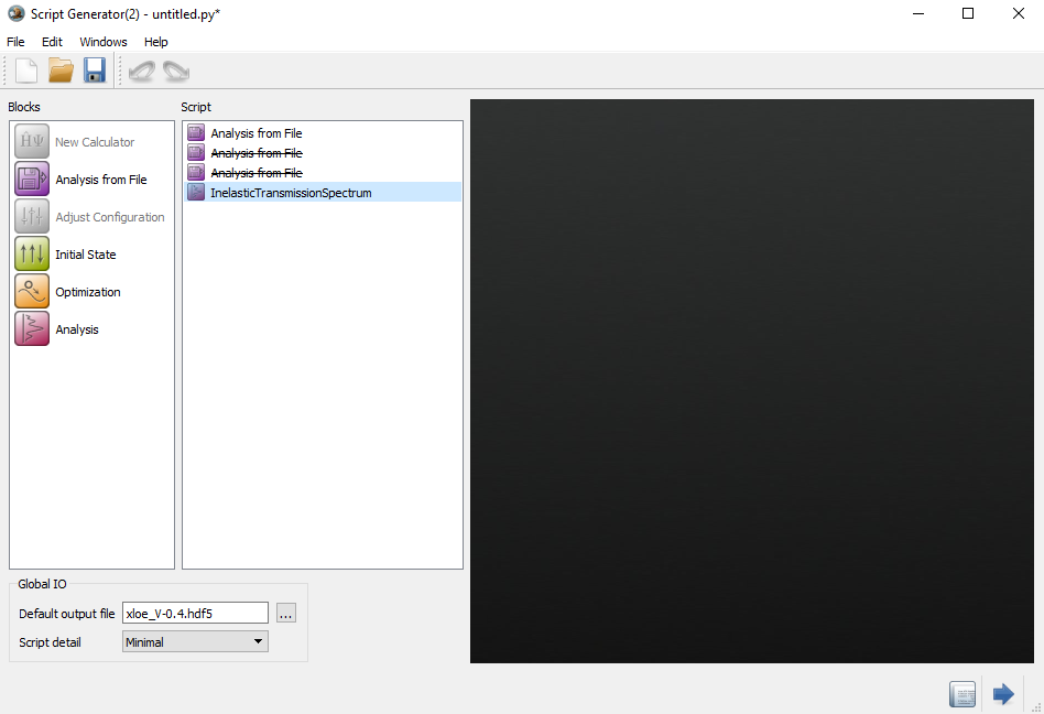
In our case, the dynamical matrix and the
Hamiltonian derivatives have already been calculated previously and can be re-used. Delete the
two blocks, add two more Analysis from File blocks and
arrange them as shown in the figure below:
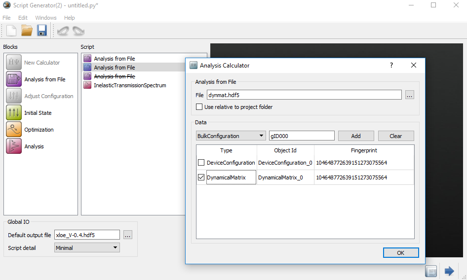
Click on the second Analysis from File block from the top.
Select the file dynmat.hdf5 and load the DynamicalMatrix object. Uncheck the
DeviceConfiguration object included in the same file. The panel should look like as in
the figure below:
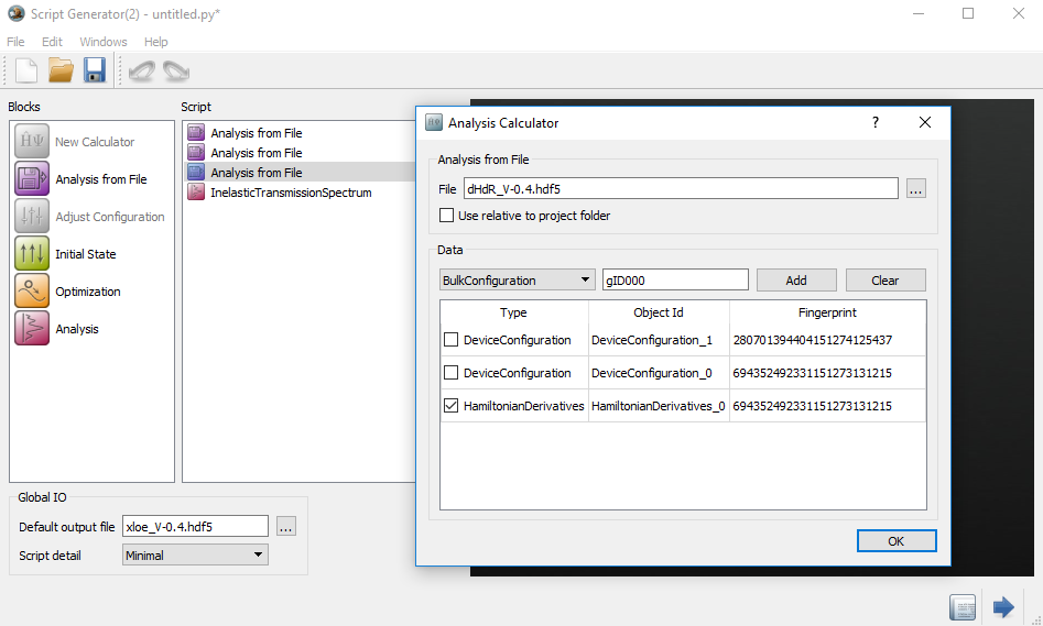
Then, click on the third Analysis from File block from the top. Select
the file dHdR_V-0.4.hdf5 and load the HamiltonianDerivatives object. The panel should
look like as in the figure below:
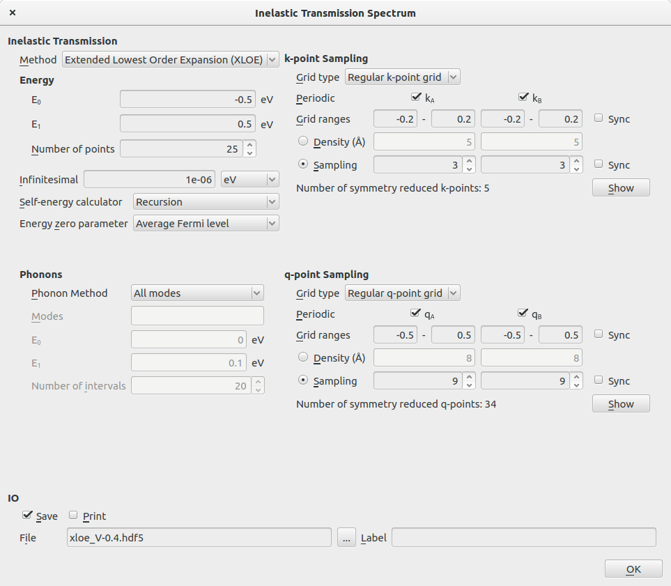
Finally, set the parameters for the Analysis ‣ InelasticTransmissionSpectrum
block as shown below:
In the Energy part, set:
\(\mathrm{E_0} = -0.5\ \mathrm{eV}\)
\(\mathrm{E_1} = 0.5\ \mathrm{eV}\)
Points = 25
In the k-point Sampling part:
set Grid type to ‘Regular k-point grid’
set the grid range for \(\mathrm{k_A}\) and \(\mathrm{k_B}\) to \([-0.2 : 0.2]\)
set the Sampling to:
\(\mathrm{k_A} = 3\)
\(\mathrm{k_B} = 3\)
In the q-point Sampling part:
set Grid type to ‘Regular q-point grid’
set the grid range for \(\mathrm{q_A}\) and \(\mathrm{q_B}\) to \([-0.5 : 0.5]\)
set the Sampling to:
\(\mathrm{q_A} = 9\)
\(\mathrm{q_B} = 9\)
In the Global IO options, change the name of the Default output file to
xloe_V-0.4.hdf5.
Send the script to the Job manager using the button,
save it as xloe_V-0.4.py and press the button to run the
calculation. The calculation will take around 1.5 hour on 24 CPUs.
You can also download the full script from here: xloe_V-0.4.py.
The results of the inelastic transmission spectrum can be analyzed in detail using the
Inelastic Transmission Spectrum Analyzer.
In the LabFloor, select the InelasticTransmissionSpectrum object contained in the file xloe_V-0.4.hdf5,
and click on the Inelastic Transmission Spectrum Analyzer plugin in the plugins panel
on the right-hand side of the screen.
First of all, you will analyze the \(\mathbf{k}\)- and \(\mathbf{q}\)-dependency of the
current. In the main window of the analyzer, set the following parameters:
Plot type : ‘Current vs. k-points’
Bias voltage : \(-0.4\ \mathrm{V}\)
You will obtain a figure similar to the one below, showing the \(\mathbf{k}\)-dependency of the
current within the sampled range of k-points. From the figure, it is evident
that the main contribution to the current comes from the \(\Gamma\)-point of the
two-dimensional Brillouin zone defined by \(k_\mathrm{A}\) and \(k_\mathrm{B}\), with
a non-negligible contribution from finite \(\mathbf{k}\)-vectors.
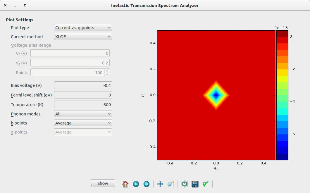
Next, change the Plot type to ‘Current vs. q-points’. You will obtain a figure similar to the one
below, showing the \(\mathbf{q}\)-dependency of the current. From the figure, it is evident
that also in this case the main contribution to the current comes from the \(\Gamma\)-point
of the two-dimensional Brillouin zone defined by \(q_\mathrm{A}\) and \(q_\mathrm{B}\),
, with a non-negligible contribution from finite \(\mathbf{q}\)-vectors.
The two figures above indicate that the current is mainly associated with transitions occurring
at the \(\Gamma\)-point of the two-dimensional Brillouin zone, both in \(\mathbf{k}\)-space and
in \(\mathbf{q}\)-space.
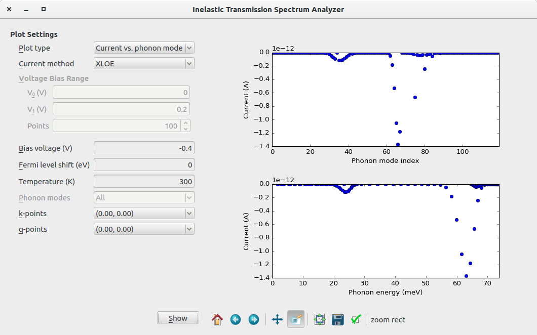
To analyze which of the phonon modes at the \(\Gamma\)-point is the one that contributes the most,
set the following parameters in the main window of the analyzer:
Plot type : ‘Current vs. phonon mode’
k-points : ‘(0.00, 0.00)’
q-points : ‘(0.00, 0.00)’
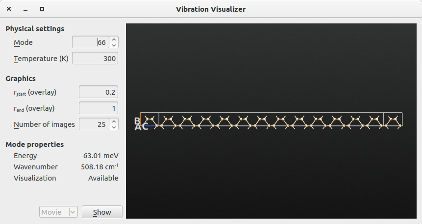
From the figure, it can be seen that the phonon that contributes the most to the current is
that with index \(66\), and energy \(\hbar \omega = 63.01\ \mathrm{meV}\).
This phonon mode can be visualized by selecting the VibrationalMode object in the file
dynmat.hdf5 calculated in Section Setting up the dynamical matrix calculation and using the
Vibration Visualizer plugin:
Note
In the figures presented above, the values of the current are negative, because the
simulations are performed in reverse bias conditions.
Calculation of the current with and without electron-phonon interactions
In order to calculate the current without and with electron-phonon interactions, download the script
current.py and run it from the terminal as:
On windows, it is not convenient to run current.py script from the terminal. In this script, you can replace filename1 and filename2 to the transmission_V-0.4.hdf5 and xloe-V-0.4.hdf5. In order to run it, drag it on the Job manager.
The script will calculate the elastic (\(I_\mathrm{el}\)) and inelastic (\(I_\mathrm{inel}\))
components of the current. The total current without and with electron-phonon interactions will then
be calculated as:
The above calculated currents are different with the currents
before analysis of the InelasticTransmissionSpectrum because of different k-points samplings.
Also in this case, the value of the current is negative, because the simulations are
performed in reverse bias conditions.
It can be seen that electron-phonon scattering leads to an increase in the
reverse bias current of about three orders of magnitude!
ATK implements several methods which can be used to speed up the calculations considerably and
enable the calculation of the inelastic transmission for devices comprised of thousands of atoms. These
methods are:
For a more detailed description of these methods, see the section Large Device Calculations of
the InelasticTransmissionSpectrum module in the ATK manual.
This method allows us to group \(3N\) phonon modes of a device with \(N\) vibrating atoms into \(M\)
energy intervals to form \(M\) new effective phonon modes, with \(M << 3N\). The inelastic transmission
spectrum will therefore be calculated only for these \(M\) effective phonon modes, greatly reducing the
computational cost of the calculation.
In the LabFloor, drag and drop the DeviceConfiguration object contained in
the file transmission_V-0.4.hdf5 to the Script generator.
Setup the calculation of the inelastic transmission spectrum as in the Calculating the inelastic transmission spectrum
Section, but in this case set the Phonon Method in the Phonons part to ‘Phonon energy intervals’.
Note
The default parameters of the Phonon energy intervals are fine for the present calculation, but
in general one should ensure that the energy range \([E_\mathrm{0}:E_\mathrm{1}]\) spans that of the
phonon modes of the calculated dynamical matrix.
In the Global IO options, change the name of the Default output file to
xloe_pheint_V-0.4.hdf5.
Send the script to the Job manager using the button,
save it as xloe_pheint_V-0.4.py and press the button to run the
calculation. The calculation will take only 20 minutes on 24 CPUs.
You can also download the full script from here: xloe_pheint_V-0.4.py.
Once the calculation is finished, run the script current.py as:
Using the bulk dynamical matrix and Hamiltonian derivatives
Another option to speed up the calculations is to use the dynamical matrix and
Hamiltonian derivatives of the bulk electrodes, instead of those of the device.
However, this is possible only for devices with a structure which is translationally
invariant along the \(\mathrm{C}\)-direction, apart from doping, electrostatic regions and
applied bias voltage.
The scripts needed to calculate the dynamical matrix and the Hamiltonian
derivatives of the bulk electrodes can be downloaded from here: dynmat_bulk.py, dHdR_bulk.py.
Running the two calculations on 4 CPUs will take less than 2 minutes.
In order to calculate the current inelastic transmission spectrum using the bulk dynamical matrix and
Hamiltonian derivatives, repeat the steps followed in Section Calculating the inelastic transmission spectrum,
with the changes described in the following.
First, click the Script generator, add the following blocks, and modify their
parameters as follows:
Analysis from File
Load the DeviceConfiguration object from the tranmission_V-0.4.hdf5 file.
Remove the DynamicalMatrix and HamiltonianDerivatives blocks, add two more Analysis from File blocks right after the Analysis from File already present, and set their properties as follows:
Click on the second Analysis from File block from the top, select the
dynamic_bulk.hdf5 file and load the DynamicalMatrix object contained in the file.
Click on the second Analysis from File block from the top, select the
dHdR_bulk.hdf5 file and load the HamiltonianDerivatives object contained in the file.
In the Global IO options, set the name of the Default output file to xloe_V-0.4_bulk.hdf5.
In this case, you need to modify the Inelastic Transmission Spectrum block in the Editor
as follows:
Send the script to the Job manager using the button,
save it as xloe_V-0.4_bulk.py and press the button to run the
calculation. Also in this case, the calculation will take only 20 minutes on 24 CPUs.
You can also download the full script from here: xloe_V-0.4_bulk.py.
Once the calculation is finished, run the script current.py as:
It can be seen that the calculated values for the current is similar to that calculated
using the dynamical matrix and Hamiltonian derivatives of the device configuration, although there
are differences due to the fact that in the present case, the loss translational invariance of the
Hamiltonian derivatives due to the applied bias is not taken into account.
 Builder, contruct the device with the following changes:
 Script generator
using the
Script generator
using the  button. Add the following blocks and set their parameters as follows:

 Job manager using the
  button to run the
calculation. It will take less than 2 minutes on 4 CPUs. You can also download the full script
from here:
button to run the
calculation. It will take less than 2 minutes on 4 CPUs. You can also download the full script
from here:  ProjectedLocalDensityOfStates object from the file
 Transmission Spectrum object from the same file and click
on the Transmission Analyzer plugin. In the plugin window, set the maximum value of the
Data range to 0.1.
Transmission Spectrum object from the same file and click
on the Transmission Analyzer plugin. In the plugin window, set the maximum value of the
Data range to 0.1.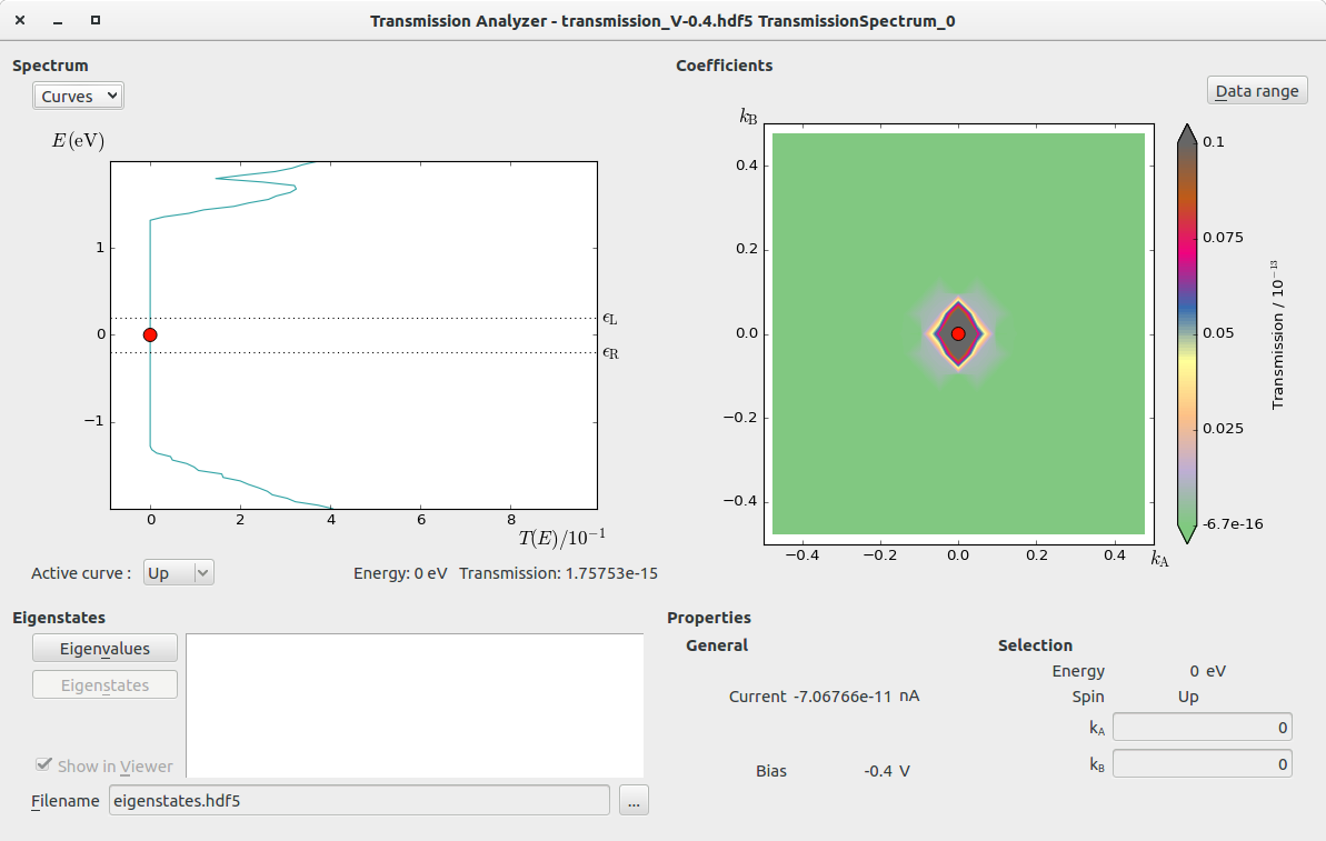

 block, select the
 InelasticTransmissionSpectrum object contained in the file
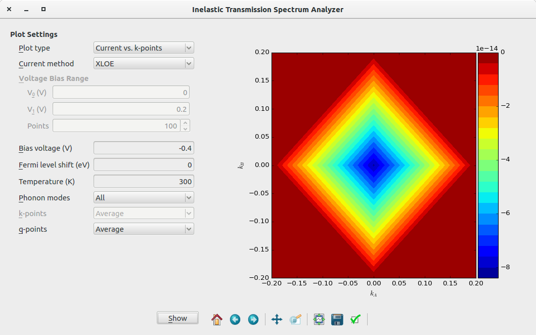


 Editor
as follows:
Editor
as follows: