Accessing QuantumATK internal variables
Version: 2016.0
The purpose of this tutorial is to illustrate how to extract internal quantities from QuantumATK. In the following, the quantities are briefly described and several sections then illustrate with examples how the information can be used to compute different sorts of transport coefficients.

Internal matrices accessible in QuantumATK
The table below lists some of the internal matrices in QuantumATK, e.g. the Hamiltonian \(H\) and the overlap matrix \(S\). The commands listed in the left-hand column in the table allow users to extract these matrices through the so-called “low level entities” module in QuantumATK.
Command |
Symbol |
|---|---|
|
\([(i,l,m),\cdots]\) |
|
\(H(\mathbf{k}), S(\mathbf{k})\) |
|
\(D(\bf{k})\) |
|
\(\Sigma^{L/R} (E,\mathbf{k})\) |
|
\(G^r (E,\mathbf{k})\) |
|
\(G^{L/R} (E,\mathbf{k})\) |
|
\(C(\mathbf{k}) , M(\mathbf{k})\) |
|
\(\Pi^{L/R} (E,\mathbf{k})\) |
|
\(D^r (E,\mathbf{k})\) |
|
\(D^{L/R} (E,\mathbf{k})\) |
You will in this tutorial see examples of how to extract these matrices and use them to compute transport coefficients. The underlying calculation engine to be used here is ATK-SemiEmpirical (ATK-SE), but could also have been ATK-DFT.
Multi-terminal conduction
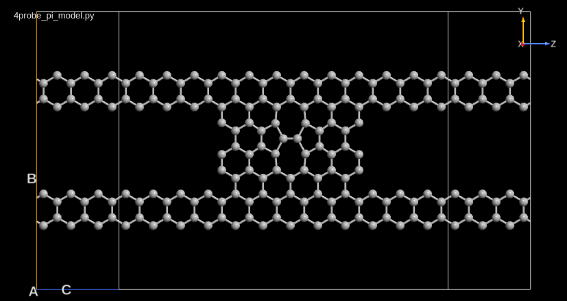
You will in this section consider a 4-probe graphene device, and calculate the transmission between each of the four probes. For the calculation, you will extract the self energies of each of the four probes and implement the Fisher–Lee transmission function in a small QuantumATK Python script. The example is inspired by the 4-probe setup in [1].
Device calculations
You should first use the Slater–Koster tight-binding method to compute the ground state and zero-bias transmission at the Fermi level for the 4-terminal graphene device illustrated below.
Start up QuantumATK with a new project, for instance named “4probe graphene”. Then download
this pre-made QuantumATK Python script and save it in the project folder: 4probe_pi_model.py. It sets
up the device configuration with a Slater–Koster calculator, and then performs the
calculation and computes the transmission at the Fermi level. All output is saved in
4probe_pi_model.hdf5.
Run the script, either using the  Job Manager or from command line:
$ atkpython 4probe_pi_model.py > 4probe_pi_model.log
The script will finish very quickly, and reports the Fermi level transmission in the log file:
+----------------------------------------------------------+
| Transmission Spectrum Report                             |
| -------------------------------------------------------- |
| Left electrode Fermi level  =  3.851459e-01 eV           |
| Right electrode Fermi level =  3.851459e-01 eV           |
| Energy zero                 =  3.851459e-01 eV           |
+----------------------------------------------------------+
   energy       T(up)
     eV
  0.000000e+00   7.553672e-01
Calculating the transmission between the 4 leads
The calculated transmission in the previous section is from the two leads on the left-hand side of the device, which are tagged “lead1” and “lead2”, to the two leads on the right-hand side of the device, tagged “lead3” and “lead4”.
Tip
You can check the tags if you send the device configuration to the  Builder.
ATK has no analysis functions for calculating transmission between individual leads. For such a calculation, you need to calculate the broadening function of each lead, \(\Gamma_i\), and then evaluate the Fisher–Lee relation,
where \(G^r\) is the retarded Green function of the device.
The downloadable script 4probe_trans.py performs this calculation. The script extracts
internal QuantumATK quantities for the calculation, and the following section discusses
details of the script.
Details of the script
The first part of the script is a utility function, which can zero out all entries
in the \(\Gamma\) matrix, except for the orbitals belonging to the indices of
the specified atoms. To obtain a list of the orbitals on the atoms, the function
uses a ProjectionList object.
# Utility function to project out Gamma of the lead1, lead2, lead3, lead4
def projectGamma(configuration, gamma, indices):
    """Zero all components in Gamma which are not in the indices list
    @param configuration : The configuration giving the full Gamma
    @param gamma         : The full gamma
    @param indices       : Indices of the atoms to project onto

    @return              : The projected gamma
    """

    projection_list = ProjectionList(indices)
    orbital_index = projection_list.orbitalIndex(configuration)
    # Make a filter matrix consisting of 1's at the orbital_index
    filter = 0*gamma
    for i in orbital_index:
        for j in orbital_index:
            filter[i,j] = 1
    return gamma*filter
Another important part is the lines shown below, which use the tags on the device configuration to determine the indices of the atoms in each electrode.
# Project onto Lead 1, 2, 3, 4
lead1_index = device_configuration.indicesFromTags('lead1')
Gamma1 = projectGamma(device_configuration, Gamma_L, lead1_index)
lead2_index = device_configuration.indicesFromTags('lead2')
Gamma2 = projectGamma(device_configuration, Gamma_L, lead2_index)
lead3_index = device_configuration.indicesFromTags('lead3')
Gamma3 = projectGamma(device_configuration, Gamma_R, lead3_index)
lead4_index = device_configuration.indicesFromTags('lead4')
Gamma4 = projectGamma(device_configuration, Gamma_R, lead4_index)
The rest of the script should be self explanatory to experienced QuantumATK users.
Running the script
Save the script and execute it. It should produce the following output:
T: L (1,2) -> R    (3,4)   : 0.756157362529
T: Up(1,3) -> Down (2,4)   : 0.232988936132

Transmission Matrix
[[ 3.99103191  0.05825146  0.04799848  0.05832079]
 [ 0.05825146  4.60578343  0.05853133  0.59130676]
 [ 0.04799848  0.05853133  3.74982393  0.05788536]
 [ 0.05832079  0.59130676  0.05788536  1.96636417]]
The script reports the transmission matrix, \(T_{ij}\). By summing up \(i \in L\), \(i \in R\) it is possible to get the transmission from left to right, which is identical (within numerical noise), to the value from the bare QuantumATK transmission calculation.
By summing up the transmission coefficients between the upper leads and the lower leads, it is possible to calculate the up-down transmission, as in [1].
Transmission projection
You will here learn how to resolve a transmission calculation into molecular projected self-consistent Hamiltonian (MPSH) eigenstates. In this way, you can analyze how large a fraction of a transmission function is propagating through a particular eigenstate or part of the system. As an example, you will investigate a dithiol-benzene (DTB) ring between two gold surfaces, see [2].

Running the calculations
Use the pre-made QuantumATK Python script au_dtb_au.py, which defines the Au–DTB–Au
device configuration, performs a DFT-SE calculation using the extended Hückel method,
and computes the Γ-point transmission in an energy range \(\pm\)1 eV around
the Fermi level. The calculations will finish in a few minutes.
Analyzing the transmission
Once the calculation has finished, the file au_dtb_au.hdf5 will appear on the
LabFloor. Select the TransmissionSpectrum item and open the Transmission Analyzer.
The Γ-point transmission spectrum has a peak 0.68 eV above the Fermi level. Select this peak using the mouse, and click Eigenvalues to calculate the transmission eigenvalues. There is one dominating eigenvalue very close to 1, and several negligible eigenvalues.
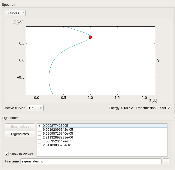
Remove the tick from all except the highest eigenvalue, and click the Eigenstates button. This will calculate the scattering eigenstate in real space, and the Viewer will pop up with a visualization of it – choose the “isosurface” visualization option if prompted. You can then use the options to tune the visualization.
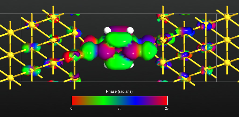
Fig. 127 Largest transmission eigenstate for energy 0.68 eV. The isosurface indicates an absolute value of 0.05 Å-3/2, and the colors indicate the phase of the eigenstate.
Projecting the transmission
We would now like to project the transmission eigenstate onto the MPSH states of the molecule, to find the orbitals that carry the transmission.
The scattering state, \(\psi(\mathbf{r})\), is expanded in basis orbitals, \(\phi_i(\mathbf{r})\), through expansion coefficients \(v_i\),
We now diagonalize the self-consistent Hamiltonian projected onto DTB,
where \(\mathbf{c}_\alpha\) are the expansion coefficients of the MPSH states.
Next, we expand the projection of the scattering state of the DTB molecule in the MPSH states,
where the expansion coefficients are given by \(a_\alpha = \mathbf{c}_\alpha^\dagger S^\mathrm{DTB} \mathbf{v}\). Through the magnitude of each \(a_\alpha\), we can get the relevance of each MPSH state, and
Below is given a script, projection.py, which calculates the largest eigenvalue scattering
state [3] at energy 0.68 eV, and calculates the projection weight of
each MPSH state,
from QuantumATK import *
from utilities import vectorToGrid, scatteringStates, averageFermiLevel
import scipy

# Read the configuration
device_configuration = nlread('au_dtb_au.hdf5', DeviceConfiguration)[0]
# Get H and S
H, S = calculateHamiltonianAndOverlap(device_configuration)
H = H.inUnitsOf(eV)

# Calculate average Fermi level
average_fermi_level = averageFermiLevel(device_configuration)
energy = average_fermi_level+0.68*eV

# Get index of orbitals on the Phenyl ring
projection_list = ProjectionList(elements = [Carbon, Hydrogen])
orbital_index = projection_list.orbitalIndex(device_configuration)
# Project H, S onto the Phenyl ring (MPSH)
H_dtb = H[orbital_index,:][:, orbital_index]
S_dtb = S[orbital_index,:][:, orbital_index]

# Calculate the mpsh eigenfunctions
w, v = scipy.linalg.eigh(H_dtb, S_dtb)

# Calculate the scattering eigenstates
T, c = scatteringStates(device_configuration, energy)

# Take the highest eigenstate
eigenvector = c[:,0]
# Project the eigenstate onto the DTB molecule
ev_dtb = eigenvector[orbital_index]
# Get the norm of the projected eigenstate
norm_ev = numpy.dot(numpy.conj(ev_dtb.transpose()), numpy.dot(S_dtb, ev_dtb))

# Loop over all MPSH
for i in range(len(w)):
    # Resolve the eigenstate into the MPSH states
    coeff = numpy.dot(numpy.conj(v[:,i].transpose()), numpy.dot(S_dtb, ev_dtb))
    # Find the strength of the MPSH projection
    p = numpy.conj(coeff)*coeff
    p = numpy.abs(p/norm_ev)
    # Print out the weight of each non negligible projection
    if p > 0.001:
        print(i, p)
The script uses some utility functions from the script utilities.py.
Running the scripts
Save both scripts, and execute projection.py using the Job Manager
or from command line. It will generate the following output:
8 0.00686834365658
11 0.00467610628863
15 0.981647336721
17 0.00670447660685
The MPSH state number 15 is clearly the one with the largest projection.
Plotting the MPSH states
The script mpsh.py shown below will save MPSH states 8, 11, 15, and 17 into the
HDF5 data file mpsh.hdf5. The script uses the function vectorToGrid(),
which performs the folding of the eigenvector with the basis functions.
from QuantumATK import *
from utilities import vectorToGrid, averageFermiLevel
import scipy

# Read the configuration
device_configuration = nlread('au_dtb_au.hdf5', DeviceConfiguration)[0]
# Get H and S
H, S = calculateHamiltonianAndOverlap(device_configuration)
H = H.inUnitsOf(eV)

# Calculate average Fermi level
average_fermi_level = averageFermiLevel(device_configuration)

# Get index of orbitals on the Phenyl ring
projection_list = ProjectionList(elements=[Carbon, Hydrogen])
orbital_index = projection_list.orbitalIndex(device_configuration)
# Project H, S onto the Phenyl ring
H_dtb = H[orbital_index,:][:, orbital_index]
S_dtb = S[orbital_index,:][:, orbital_index]

# Calculate the eigenfunctions
w, v = scipy.linalg.eigh(H_dtb, S_dtb)
# Calculate eigen energies relative to the fermi level
eigen_energies =  (w*eV-average_fermi_level)

# Save eigenstates number 13-17
for i in [8, 11, 15, 17]:
    print('eigenenergy ', i,  eigen_energies[i])
    # Put the eigenvector into a vector of length of all orbitals
    number_orbitals = H.shape[0]
    eigenvector = numpy.zeros(number_orbitals, dtype=complex)
    eigenvector[orbital_index] = v[:,i]
    grid = vectorToGrid(eigenvector, device_configuration)
    nlsave('mpsh.hdf5', grid)
Run the script, and when finished drag and drop the object with ID gID002
from mpsh.hdf5 onto the  Viewer. Then add the device configuration
to the plot by drag and dropping it from
Viewer. Then add the device configuration
to the plot by drag and dropping it from au_dtb_au.hdf5. By adjusting the
plot properties, you should be able to get the image shown below.
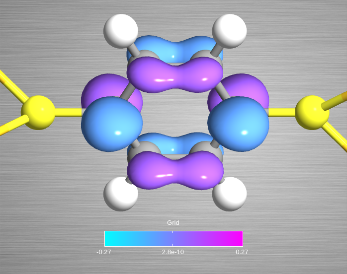
Fig. 128 Isosurface with isovalue 0.07 Å-3/2 for MPSH state number 15.
Note
The vectorToGrid() method uses a finer grid spacing than the value set by
the HuckelCalculator. This is why the image above has high-quality resolution.
AC conductance
The scripts presented in this section can be used to calculate the AC conductance of a nanodevice within the wide-band limit. The implementation follows closely the work by Yamamoto et al. [4].
We will here consider the (10,10) carbon nanotube device illustrated below, and use
again the extended Hückel method with a \(\pi\)-model. Use cnt_device.py to perform
the ground state device calculation.
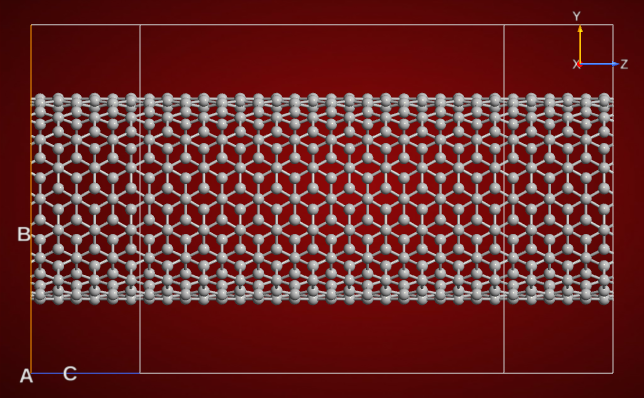
Fig. 129 (10,10) CNT device configuration with a central region length of 24.61 Å.
The admittance is defined as the inverse of the impedance, and is a measure of
how easily a device will allow a current to flow. Download the scripts cnt_admittance.py
and admittance.py to your QuantumATK project folder. Then execute cnt_admittance.py, which computes
and plots the real (G) and imaginary (B) parts of the AC admittance for the CNT
device.
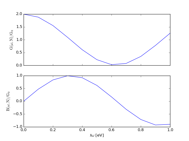
Fig. 130 Real (G) and imaginary (B) parts of the AC admittance for a (10,10) CNT device.
Note
Since the implementation of the AC conductance is done in Python and uses dense matrices, the calculation is computationally inefficient, and for systems with a large number of orbitals the calculation can take substantial time.