Spin-dependent Bloch states in graphene nanoribbons
Version: 2017
Graphene nanoribbons (GNRs) are very interesting systems for novel electronics applications. Depending on the shape of the ribbon edge, the ribbons can have metallic or semiconducting characteristics. As we will see in this tutorial, spin also plays an important role for the transport properties of GNRs.
You will use the capabilities of QuantumATK and ATK to study the spin-dependent bandstructure of a zigzag GNR. These ribbons are metallic if the calculation is performed without accounting for spin, but when spin is included, a band gap opens up. By plotting conduction and valence band Bloch states for various k-points, You will see how the two spin-components are localized on opposite sides of the ribbon.
Note
This tutorial will involve calculations that take at most 5-10 minutes on a usual laptop, so there is no real need to use a separate, more powerful computer or to run the jobs in parallel.
It will be assumed that you are familiar with the basic operations in the software corresponding to the level of experience gained from completing the basic QuantumATK Tutorials. No proficiency in programming will be necessary.
Band structure of a zigzag nanoribbon
We will begin by constucting a graphene zigzag nanoribbon and calculate the bandstructure. Spin will be added in the next section.
Constructing the Graphene Nanoribbon
Start QuantumATK, create a new project and give it a name, then select it and click
Open. Launch Builder by clicking the Builder icon  on the tool bar.
In the Builder, click . This launches the Graphene Ribbon builder tool.
Leave all parameters at their default values and click Build.
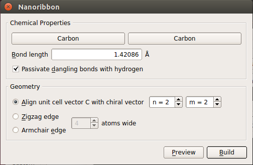
The repetition is automatically set to the minimal value. This reduces calculation time and makes it easier to analyze the band structure.
There are periodic boundary conditions perpendicular to the ribbon, and the unit cell padding distance is automatically set to 10 Å, to reduce any residual electrostatic interactions with the periodic images of the ribbon.
Calculating the graphene band structure
Now send the structure to the Script Generator by clicking the “Send To”
icon  in the lower right-hand corner of the window, and select
Script Generator (the default choice, highlighted in bold) from the pop-up
menu.
in the lower right-hand corner of the window, and select
Script Generator (the default choice, highlighted in bold) from the pop-up
menu.
In the Script Generator,
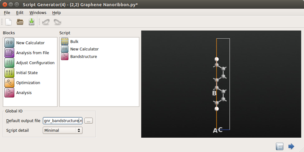
Add a New Calculator block
.
Add an block
.
Change the default output filename to
gnr_bandstructure.hdf5.
The Script Generator should now look like this:
Open the New Calculator by double-clicking it.
Most of the default parameters are good enough, but a few of them need adjustment.
You must carefully consider the k-point sampling. Since the unit cell along the ribbon is quite short, there must be a large number of k-points along the C-direction (along the ribbon).
Select 50 k-points in the C-direction.
This is a good trade-off between calculation time and accuracy. You only need a single point along the transverse A- and B-directions, since the system is not periodic in these directions.
Next, under Calculator settings, choose Basis set/exchange correlation and reduce the basis set to SingleZetaPolarized for each element in the box on the lower right. This is to gain some speed; for this particular system, that level of accuracy is sufficient.
The calculator dialog should now have the following settings
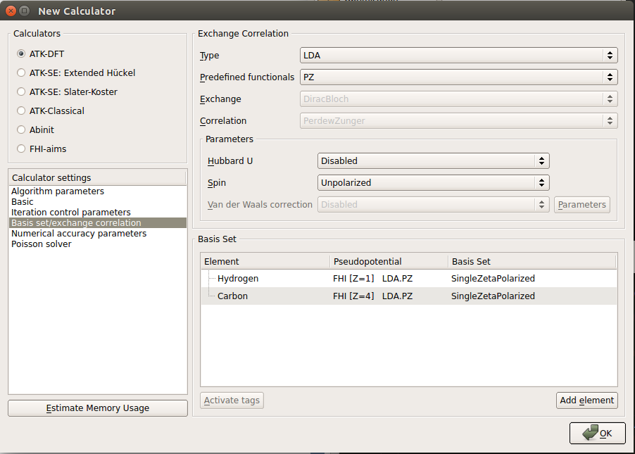
Finally, click the OK button.
To specify the band structure calculation, double-click the Bandstructure block.
In the appearing dialog, change Points pr. segment to 200. This implies that each band will be calculated with a resolution of 200 points. Also notice that the default suggested route in the Brillouin zone (from G (0,0,0) to Z (0,0,1/2)) is the appropriate one.
Note
The label “G” is used in ATK (and QuantumATK) to designate the \(\Gamma\) point, when setting up the script. In the band structure plot, the proper Greek label will be shown (see below).
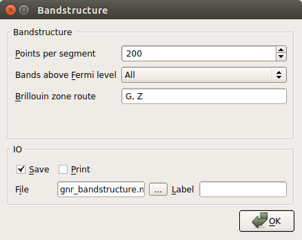
Finally, click the OK button.
Now run the calculation by clicking the Send To icon and
select Job Manager from the pop-up menu. Save the Python script under an
appropriate name, such as gnr_bandstructure.py and click OK.
In the Job Manager, click the Start icon  to run the
job; the calculation takes only seconds to complete.
to run the
job; the calculation takes only seconds to complete.
Analyzing the results
Return to the main QuantumATK window. The file gnr_bandstructure.hdf5 should
now be visible under “Project Files” in the left column. In the middle column,
called the LabFloor, select Group by Item Type.
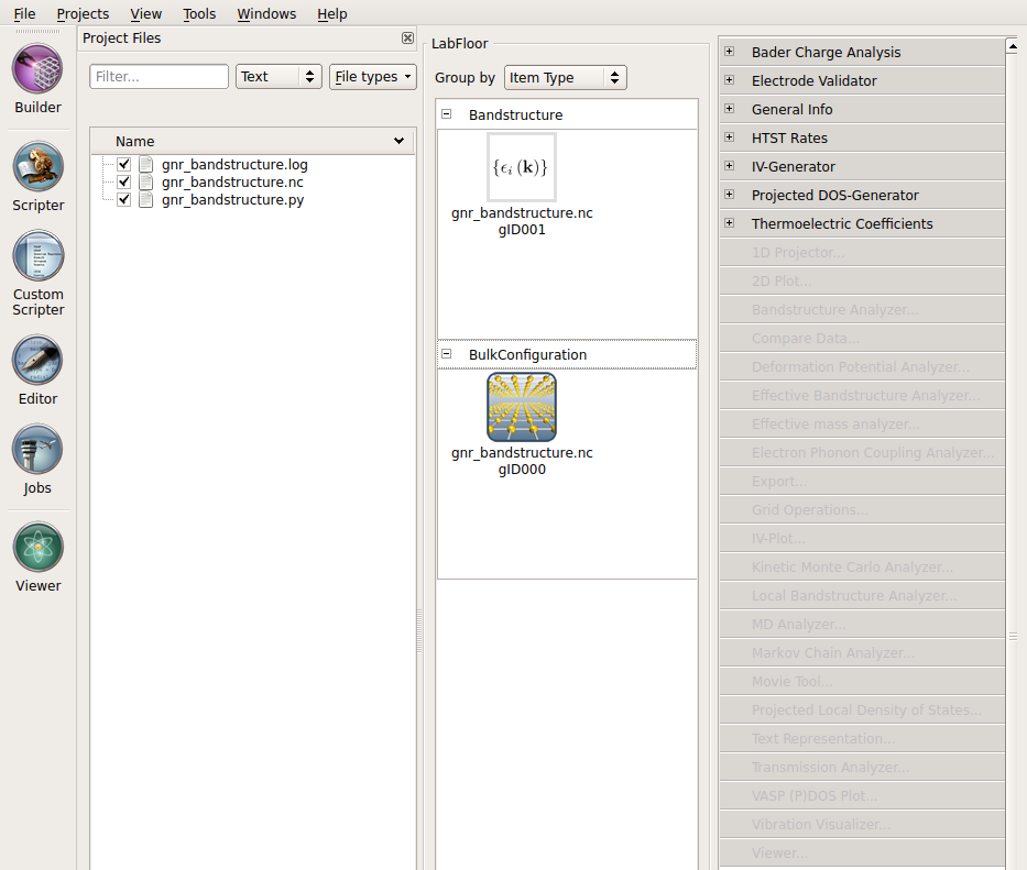
On the LabFloor, you can see that the file contains two objects: the calculated Bandstructure and the BulkConfiguration itself. The latter object contains not only the geometry, but the full state of the calculation. We will use this in the next chapter to calculate the Bloch functions without having to rerun the self-consistent calculation. For this, you will need to know the Id of the BulkConfiguration, which is shown after the file name; it is gID000 in this case.
Now, to plot the band structure, select the Bandstructure object (gID001), and click the Bandstructure Analyzer button in the plugin panel on the right.
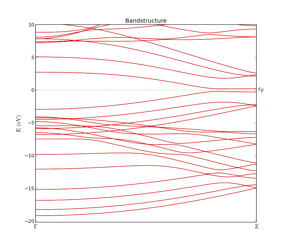
The resulting plot is shown in the figure below. Note how the conduction and valence bands stick together for high values of kz. This is a characteristic feature of zigzag ribbons (in our model) and clearly makes our ribbon metallic.
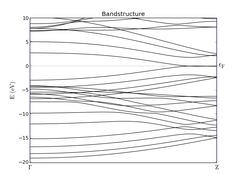
Fig. 99 Band structure of a zigzag graphene nanoribbon. The band gap at the \(\Gamma\)- point is roughly 5 eV, but closes entirely at the Z-point.
Bloch states
A very useful feature in ATK is its ability to calculate and plot Bloch states, which can be used to investigate the symmetry of certain bands and how this may relate to the transport properties. You will now use this capability to see how Bloch states close to the \(\Gamma\) point are delocalized across the ribbon, while states with higher kz become increasingly localized towards the edges.
The ribbon consists of 8 carbon and 2 hydrogen atoms in each unit cell. A carbon atom contributes four valence electrons (2s22p2 ) and hydrogen only one (1s). Thus there are 34 electrons in the system. Each band is doubly degenerate (due to spin) and hence there will be 17 valence bands. Counting from 0, the band index of the highest valence band is 16 and the index of the lowest conduction band will be 17.
Setting up the calculation
You will now set up a script that computes the Bloch functions of these two
bands, in three different k-points. The self-consistent state of the ribbon
was saved in the file gnr_bandstructure.hdf5, and you can just restore
it for this analysis, instead of rerunning the self-consistent loop. This is a
very convenient way to separate the actual self-consistent calculation, that
you perhaps prefer to run on a cluster (at least for a bigger system), and the
subsequent analysis that often requires less resources and can be run directly
via the Job Manager in QuantumATK.
From the main QuantumATK window, launch Script Generator by clicking the Script Generator icon
.
The double-click the Analysis from File icon
(it is the only available choice when we start the Script Generator in this way and without dropping a configuration on it).
Double-click the icon and specify the file name
gnr_bandstructure.hdf5in the appearing dialog.You should also specify the object ID of the configuration in this file you want to use for the analysis. As we found out in the previous chapter, this is gID000 for our case (it usually is, if the HDF5 file only contains one configuration).
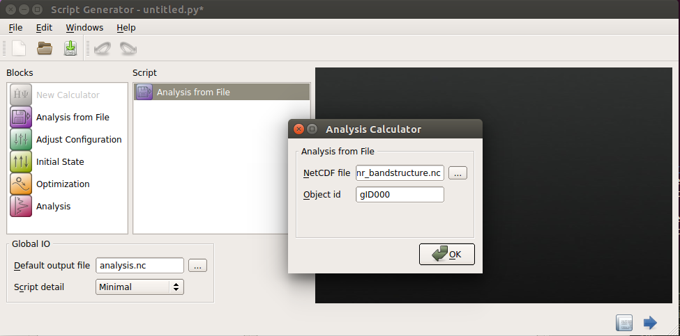
Then click the OK button.
Now, we need to set up the calculation of the Bloch states.
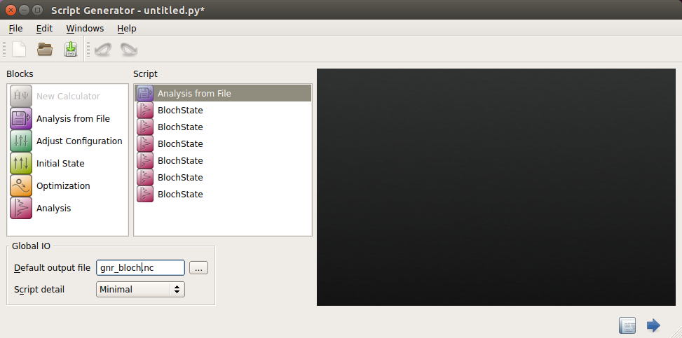
Add 6 times. This should give 6 BlochState icons
Change the output file to
gnr_bloch.hdf5.
The Script Generator window now loooks as follows:
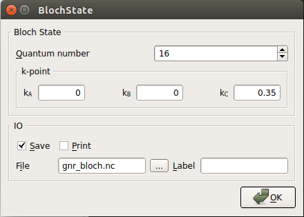
Double-click each of the first three Bloch state icons, enter 16 as the Quantum number (i.e. the band index), but give each one different k-points:
(0, 0, 0)
(0, 0, 0.35)
(0, 0, 0.5)
In the second case, the BlochState window should look like the one shown below:
Repeat this procedure for the three remaining Bloch state icons, but this time enter 17 as the value for the Quantum number.
Finally, like before, send the job to the Job Manager and start the execution of the job.
Note
The calculation is very fast, but the generated HDF5 file will be quite large (about 120 Mb), which is why the data is saved in a separate file. This way, we avoid bloating the original file containing the self-consistent calculation (which would make it slower to read, if you desire to do some other analysis).
Analyzing the results
Once the job finishes, return to the main QuantumATK window. The results from
gnr_bloch.hdf5 should automatically be included in the LabFloor (see
that the gnr_bloch.hdf5 is checked under the under Project Files).
Select Group by Item Type and expand the BlochState block.
Click on the last (gnr_bloch.hdf5 gID005) of the six BlochState objects
and select Viewer and then make sure the Plot type is set to Isosurface
before pressing OK. Do this for each of the others, continuing with
gID004, until all 6 are shown in the Viewer window. Now, select
from the menu at the top of the Viewer
window, in order to arrange the plots neatly. Note that the plots are now
arranged with the newest window in the upper left corner, meaning that we have
the valence band in the top row and the conduction band in the bottom row,
with the gamma point to the left and the Z point on the right.
Tip
You may also add the subsequent Bloch state objects to the Viewer window by drag-and-drop. However, in this case you need to make sure that you do not drop the objects on an existing plot, as it will then be added to this instead of being created as a separate plot.
To adjust the properties of each plot, click Properties from the menu on the right. This must be done separately for each window.
Under Isosurface (the first tab), set the Isovalue to 0.05 and select the HSV color map.
You can also go to the Scene tab and hide the axes by removing the tick from Compass enabled.
Below the visualization of the 6 different Bloch states are shown in the viewer. The quantum number is 16 for the top three and 17 for the bottom three, and the k-point coordinates are: (0,0,0), (0,0,0.35) and (0,0,0.5), starting from the left.
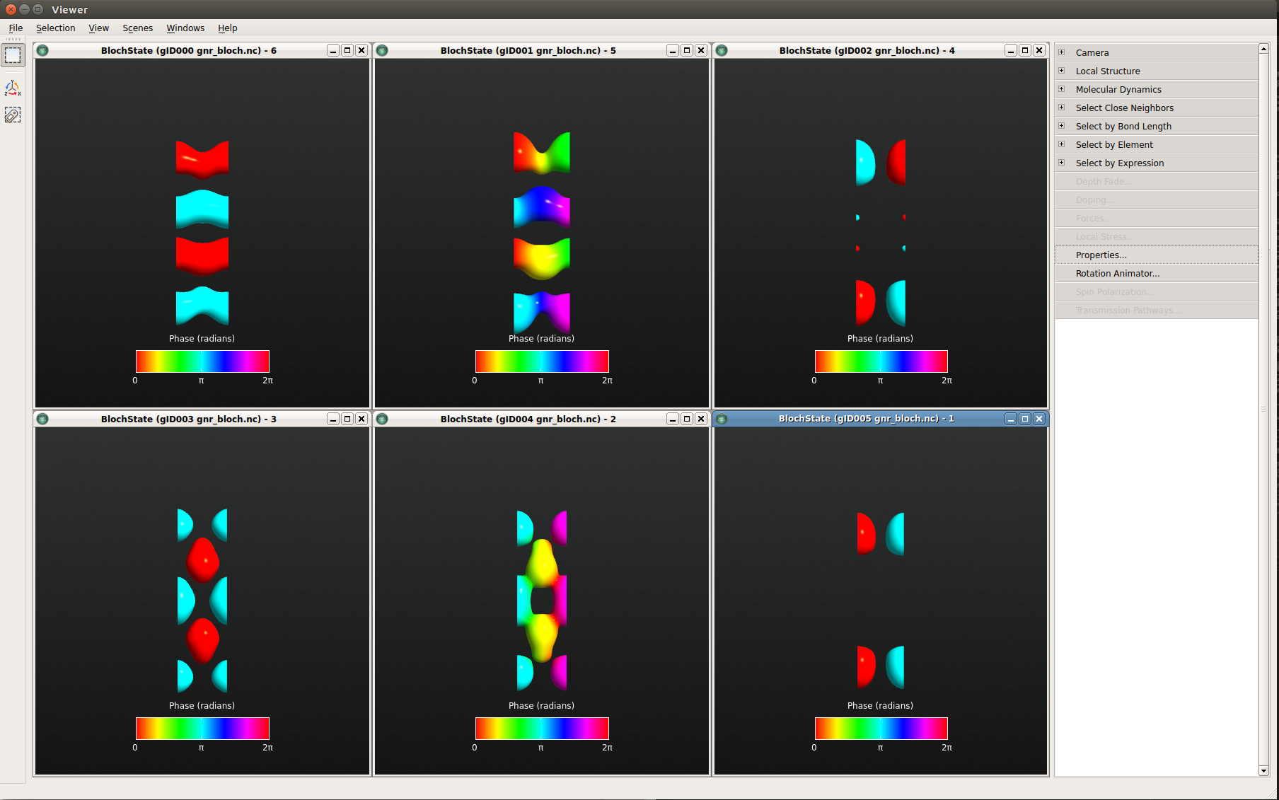
Fig. 100 From left to right: The \(\Gamma\) point, k=0.35, and the Z point. The top and bottom rows display the valence and conduction bands, respectively. (You may obtain a phase shift of \(\pi\) in your figures compared to this image; this has no physical relevance, of course.)
Looking at the respective Bloch functions, first note that the wave functions at G and Z are real (as expected), and second that there is a distinct difference between valence and conduction band Bloch functions. The occupied valence band states appear to be “connected” in the ribbon direction, while the (unoccupied) conduction band states are more oriented across the ribbon. At Z, the states become localized towards the edges of the ribbon.
In the next section, you will see how spin splits the degeneracy around Z, and how the two spin states become localized on opposite edges.
Tip
To superimpose the geometry of the ribbon on the plot, drag the
BulkConfiguration object from the file gnr_bandstructure.hdf5 onto a
BlochState window in the open Viewer window.
Introducing spin
Setting up the calculation
You will now redo the entire calculation with spin-polarization included. The work-flow is very similar, and each step is therefore only outlined this time.
Set up the calculation like you did for the bandstructure calculation: Go to the builder and send the graphene nanoribbon to Script Generator (the builder stash should still contain the graphene nanoribbon from last time).
Add a New Calculator block and set the same parameters as before (SingleZetaPolarized basis set and (1,1,50) k-points). In addition, in the New Calculator dialog window, set Spin to Polarized and check that the exchange-correlation functional has automatically changed to LSDA.
The default in ATK is to start a spin-polarized calculation with a symmetric initial spin density. However, in this case, this will result in a local minimum corresponding to a symmetric (ferromagnetic) state. To get the real anti-ferromagnetic ground state of the graphene nanoribbon we have to set up the initial spin configuration with opposite polarizations on the two nanoribbon edges (the middle carbon atoms and the hydrogen can be left “unpolarized”).
To set up the initial spin state of the system:
Double-click the Initial State icon
to add it and then open it.
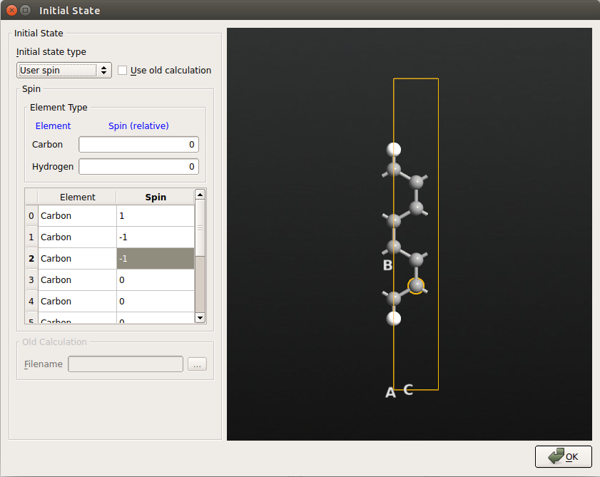
Set Initial state type to “User spin”, and then under Spin, set the default spin of both carbon and hydrogen to 0.
Then in the 3D view, select (by using Ctrl+left-mouse click) the two upper carbon atoms and verify that their numbers are 0 and 7 in the list. Set their spin values to 1. Repeat this procedure for the two lower carbon atoms (they should be number 1 and 2 in the list) setting their initial values to -1. The hydrogen atoms and the four middle carbon atoms can be left with spin values equal to 0. The Initial State dialog now look as shown below: (don’t be confused by the fact that the carbon atoms are not ordered by Y coordinate).
Tip
If you have no idea about the spin state of the system, you may select Random spin. It sets a random spin on each atom, and dependent on the random values, the system may converge to different spin states of the system. The spin state with lowest total energy is the ground state.
Add a Bandstructure calculation for the spin polarized calculation and again set Points pr. segment to 200.
This time, you may just as well include the Bloch states from the beginning to get everything done in one script. For the following analysis, it is sufficient to only calculate the Bloch functions in the Z point. Add two Bloch state icons all defined at the Z point (0,0,1/2). Let one of these have Quantum number 16 and the other have the Quantum number 17.
We will also need the electron density later, so add also an object.
Another way to look at the spin density is through the Mulliken populations, so add also an object.
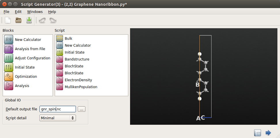
Then set the name of the output file for the calculation in the Script Generator window to
gnr_spin.hdf5. The Script Generator window should now look like the one shown below.
Send the script to the Job Manager and run the calculation.
Analyzing the results
By inspecting the column “DD” in the calculation log you will see, by summing the entries, that there is no total spin-polarization in this system (the total spin up and down will both be 17), which is very reasonable; carbon is not magnetic.
By plotting, you can also observe that there is no spin-dependence in the band structure; the up and down states are completely degenerate (otherwise you would see both blue and red curves in the band structure plot).
However, the inclusion of spin does have a profound effect on the bandstructure. The earlier degeneracy of the conduction and valence bands close to kz =0.5 is broken, and a band gap has opened up.
Plot the corresponding Bloch states at the Z point and select to plot spin up and down for each of the two BlochState objects. If you adjust the view properties as in the previous chapter, you clearly see how the two spin valence states are localized on opposite edges of the ribbon. The conduction band states behave completely analogously, but are localized on opposite edges compared to the valence band states.
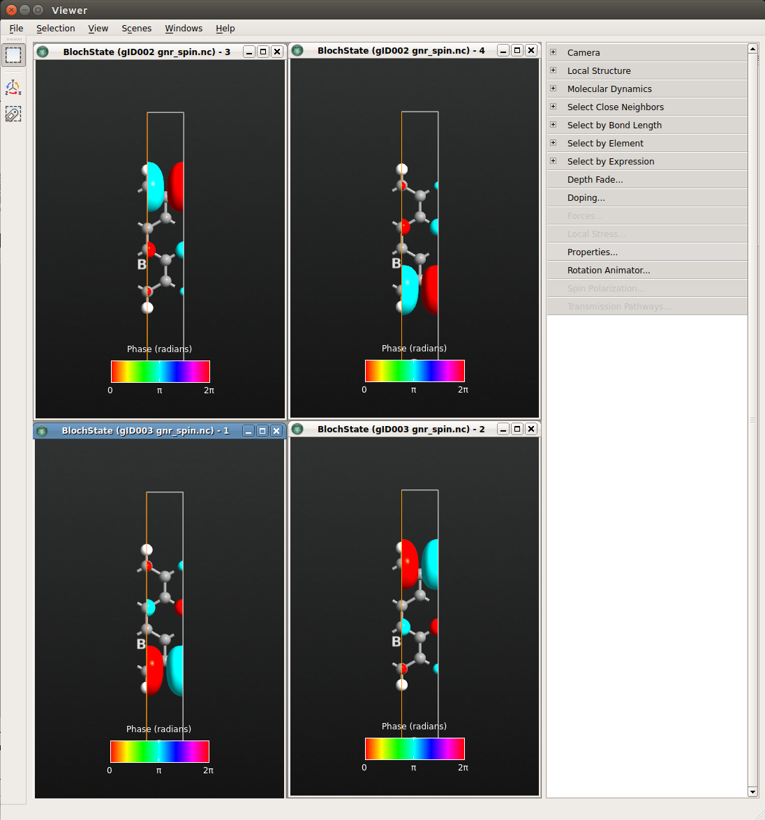
Fig. 101 Spin up (right) and down (left) states at the Z point for the highest valence band (bottom) and lowest conduction band (top).
Electron density and Mulliken populations
Since the up and down Bloch states are localized on opposite edges, there must be a difference in the total spin up and down electron density.
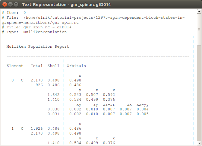
The Mulliken populations is the easiest way to get a first view of this, and it is most conveniently viewed by selecting the MullikenPopulation object on the LabFloor and selecting Text Representation… on the right. The resulting window is shown below. Under the column “Total”, the two spin-channels are shown on seprate lines, and we find that the two edge carbon atoms (numbers 0 and 1) have a surplus population of 0.25 of either spin-up or spin-down.
You can also choose to plot the spin difference density, \(\rho_{\uparrow} - \rho_{\downarrow}\), or the normalized difference between the spin up and down density, (\(\rho_{\uparrow} - \rho_{\downarrow}) / (\rho_{\uparrow} + \rho_{\downarrow}\)).
All the information you need is contained in the ElectronDensity object saved
in the gnr_spin.hdf5 file.
Plotting the spin density
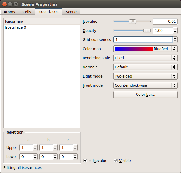
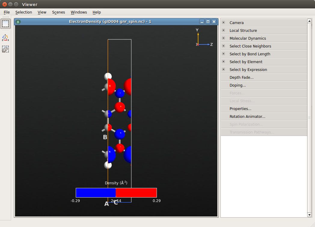
First we plot the direct spin difference density. Select the ElectronDensity object on the LabFloor and click Viewer. Go to properties and set the Isovalue to 0.01, the Color map to BlueRed and check the box for \(\pm\) Isovalue at the bottom. The window should now look as the one shown below.
If you also overlay the bulk configuration as explained previously, you should get a plot like the one shown below.
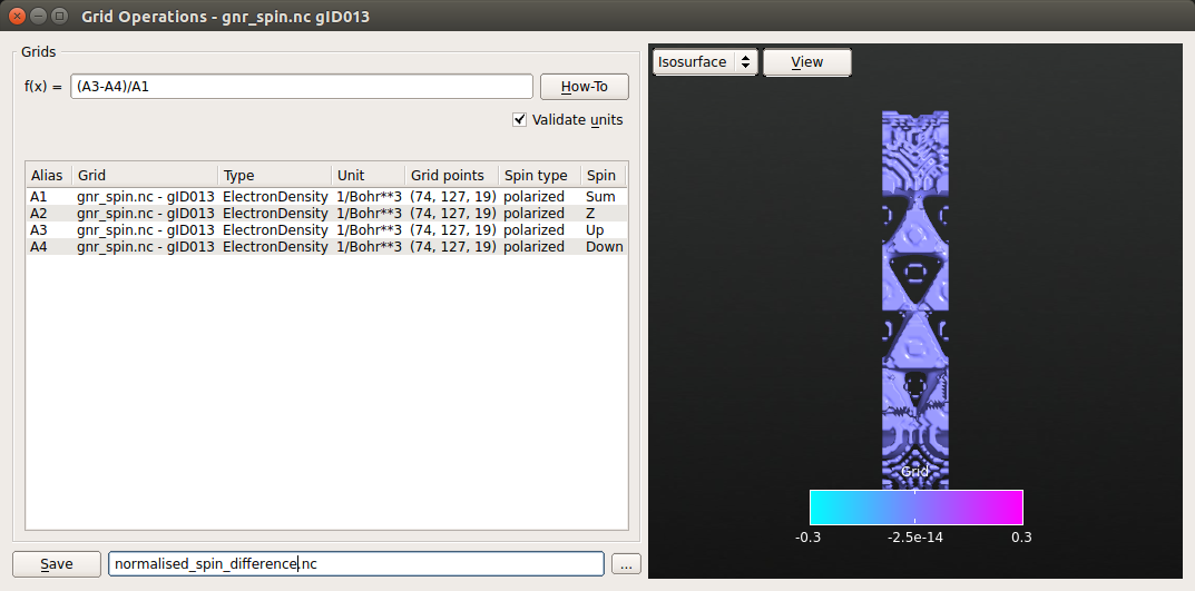
In order to plot the normalised spin difference density, go to LabFloor and
select ElectronDensity in the gnr_spin.hdf5 file and click on
Grid Operations. Here, you can see the elements that are contained in the
ElectronDensity object which are marked by an alias. In the f(x) field you
can now write any mathematical expression. In this case write (A3-A4) / A1.
Finally, save the result in a new file called
normalized_spin_difference.hdf5.
Note
You can select more then one object present in the LabFloor by holding Ctrl and click on Grid Operations. In this way you will be able to operate on different data set from different calculations. However, note that the dimensions of the grids must be the same and the units of the grids in the expression must be consistent.
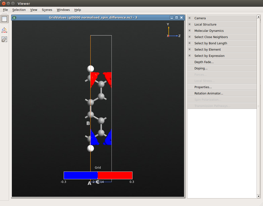
The new file will appear in the LabFloor. Select it and plot the content with the Viewer. In order to get a better view, open Properties on the menu in the right-hand side. Again, check \(\pm\) Isovalue at the bottom, change Isovalue to 0.02 in the upper right and change the color map to BlueRed.
You can also average the spin polarization along the x-axis (perpendicular to the graphene sheet). The following script will generate the plot below, using the matplotlib module which is integrated in ATK.
Drop the script on the Job Manager, and it will generate the plot. The plot
will be saved in the file av.png.
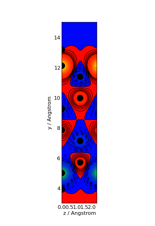
Fig. 102 Averaged spin polarization density. The filled circles indicate the atom positions.