NEGF: Device Calculators
Introduction
This section describes the most important aspects of the formalism in QuantumATK for simulating device systems using the non-equilibrium Green’s function (NEGF) method. For a more detailed description of the theory and application examples you may consult QuantumATK reference paper by Smidstrup et al. [1] and some of the many research papers on the subject [2], [3], [4], [5].
In QuantumATK, the NEGF formalism is implemented in combination with DFT: LCAO and Semi Empirical in the DeviceLCAOCalculator and the DeviceSemiEmpiricalCalculator, respectively.
Device configuration
A typical device configuration is illustrated in Fig. 157.
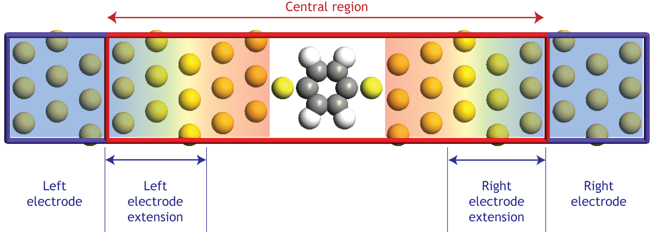
Fig. 157 Geometry of a device configuration with two electrodes (two-probe configuration). In the left and right electrode regions the system is periodic in the transport direction (the C direction). The central region seamlessly connects the left and right electrode regions, and the part of the central region where the atom positions follow the periodic arrangement of the electrodes is called the left and right electrode extension. The background color symbolizes the perturbation of the electrode effective potential relative to the electrode self-consistent value. A sufficient fraction of the electrodes must be included in the central region to screen out the perturbation of the scattering region, such that the outermost part of the central region attains an effective potential similar to the bulk potential of the electrodes. The matching between these potentials forms the boundary condition for the electrostatic problem.
The system can be divided into three regions: left, central, right. The implementation relies on the so-called screening approximation, which assumes that the properties of the left and right regions, the electrodes, can be described by solving a bulk problem for the fully periodic electrode cell. The screening approximation will formally be fulfilled when the current through the system is sufficiently small that the electrode regions can be described by an equilibrium electron distribution.
Fig. 157 illustrates how the electrode regions must be extended into the central region, in order to screen out the perturbations from the scatterer (in this case the benzene molecule) inside the device. For metallic electrodes it is usually sufficient to extend the electrodes 5-10 Å into the central region.
Non-equilibrium electron distribution
The left and right regions are equilibrium systems with periodic boundary conditions, and the properties of these systems are obtained using a conventional electronic structure calculation. The challenge in calculating the properties of a device system lies in the calculation of the non-equilibrium electron distribution in the central region.
The assumption is that the system is in a steady state such that the electron density of the central region is constant in time. The electron density is given by the occupied eigenstates of the system. Since the chemical potential is different in the two electrodes, the contribution from each electrode to the total electron density in the central region must be calculated independently:
The contribution from the left (\(n^L\)) and right (\(n^R\)) electrodes can be obtained by calculating the scattering states, which are the eigenstates of the system when scattering boundary conditions are used. Fig. 158 illustrates a left moving scattering state with origin in the right electrode.
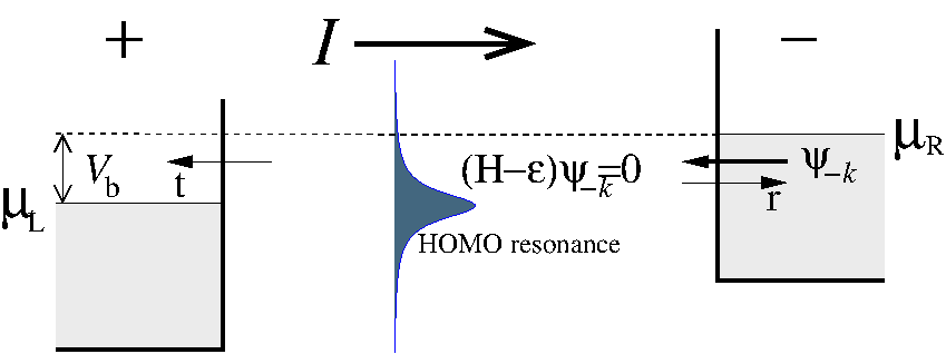
Fig. 158 The electron distribution in a device configuration. The left and right regions have an equilibrium electron distribution with chemical potentials \(\mu_L\) and \(\mu_R\), related through the applied sample bias, \(\mu_R - \mu_L = e V_b\) . The electrons with energies in the bias window \(\mu_L \leq \varepsilon \leq \mu_R\) , give rise to a steady state electrical current. The figure illustrates a left moving scattering state with origin in the right electrode.
The left and right density are now calculated by summing up the occupied scattering states,
The scattering states of the system are calculated by first calculating the Bloch states in the electrodes and subsequently solving the Schrödinger equation of the central region using the Bloch states as matching boundary conditions.
The non-equilibrium Green’s function (NEGF) method
Instead of using the scattering states to calculate the non-equilibrium electron density, QuantumATK uses the non-equilibrium Green’s function (NEGF) method; the two approaches are formally equivalent and give identical results [2].
The electron density is given in terms of the electron density matrix, as described in section Electron density. We divide the density matrix into left and right contributions,
The left density matrix contribution is calculated using the NEGF method as [2]
where
is the spectral density matrix. Note that while there is a non-equilibrium electron distribution in the central region, the electron distribution in the electrode is described by a Fermi function \(f\) with an electron temperature \(T_L\) .
In this equation, \(G\) is the retarded Green’s function, and
is the broadening function of the left electrode, given in terms of the left electrode self energy, \(\Sigma^L\) . A similar equation exists for the right density matrix contribution.
The following section describes the calculation of \(G\) and \(\Sigma\) in more detail.
Retarded Green’s function
The key quantity to calculate is the retarded Green’s function matrix,
where \(\delta_+\) is an infinitesimal positive number. \(S\) and \(H\) are the overlap and Hamiltonian matrices, respectively, of the entire system.
The Green’s function is only required for the central region and can be calculated from the Hamiltonian of the central region by adding the electrode self energies:
Therefore, the calculation of the Green’s function of the central region at a specific energy requires the inversion of the Hamiltonian matrix of the central region. In QuantumATK this matrix is stored in a sparse format, and the inversion is done using an \(\mathcal{O}(N)\) algorithm [6].
Self energy
The self energy describe the effect of the electrode states on the electronic structure of the central region. The self energy can be calculated from the electrode Hamiltonian. QuantumATK provides 4 different methods for calculating the self energy:
DirectSelfEnergy uses an exact diagonalization of the Hamiltonian for calculating the self energy [7].
RecursionSelfEnergy uses an iterative scheme for calculating the self energy [8], which gives essentially the same results as the direct method but is faster for some systems.
SparseRecursionSelfEnergy uses the same iterative scheme as RecursionSelfEnergy, but exploits inherent sparsity. This provides a smaller memory footprint, as well as increased performance for all but the smallest systems.
KrylovSelfEnergy is an approximate method which is an order of magnitude faster that the other methods, but may in rare cases give inaccurate results [9], [10] .
Complex contour integration
The energy integral needed to obtain the density matrix within the NEGF framework is evaluated through a complex contour integration. It is divided into two parts; an integral over equilibrium states and an integral over non-equilibrium states.
The integral over the equilibrium states can be done using two different methods:
SemiCircleContour: Defines a semi-circular complex contour that gives high computational efficiency [2].
OzakiContour: Evaluation of the complex contour integral is based on the residue theorem and a continued-fraction representation of the Fermi–Dirac districution [11][12]. This is a highly stable method, but is also less efficient than SemiCircleContour.
The integral over the non-equilibrium states must be performed along the real axis, and uses the RealAxisContour method. Note that for large biases, this is often the most demanding part of the calculation.
Lastly, one of two different contour methods must be chosen (usually just left at the default value):
SingleContour uses a single contour for the calculation. This is appropriate for small biases, and is the fastest method.
DoubleContour uses a double contour for the calculation. This gives best stability and must be used for high biases. The method can also handle if there are bound states inside the bias window.
See also ContourParameters.
Spill-in terms
In terms of the density matrix, \(D\) , the electron density of the central region is given by
The Green’s function of the central region gives the density matrix of the central region, \(D_{CC}\) , however, to calculate the density correctly close to the central cell boundaries the terms involving, \(D_{LL},D_{LC},D_{CR},D_{RR}\) are also needed. These terms are denoted spill-in terms [13].
ATK includes all the spill-in terms, both for calculating the electron density \(n ({\bf r})\) and the Hamiltonian integral. This gives additional stability and well-behaved convergence in the device algorithm [13].
Effective potential
Once the non-equilibrium density is obtained the next step in the self-consistent calculation is the calculation of the effective potential as the sum of the exchange-correlation and electrostatic Hartree potentials. The calculation of the exchange-correlation potential is straightforward since it is a local or semi-local function of the density. However, the calculation of the electrostatic Hartree potential requires some additional consideration for a device system. The following describes the calculation of the Hartree potential in more detail.
The starting point is the calculation of the self-consistent Hartree potential in the left and right electrodes. The Hartree potential of a bulk system is defined up to an arbitrary constant. However, in a device setup the Hartree potentials of the two electrodes are aligned through their chemical potentials (i.e. their Fermi levels), since these are related by the applied bias:
The Hartree potential of the central region is obtained by solving the Poisson equation, using the bulk-like Hartree potentials of the electrodes as boundary conditions at the interfaces between the electrodes and the central region. An overview of the available Poisson solvers and how boundary conditions are applied for NEGF calculations is given in Boundary conditions.
Total energy and forces
A device system is an open system where charge can flow in and out of the central region from the left and right reservoirs. Since the particle number is not conserved it is necessary to use a grand canonical potential to describe the energetics of the system [14]:
where \(N_{L/R}\) is the number of electrons contributed to the central region from the left/right electrode.
Due to the screening approximation, the central region will be charge neutral, and therefore \(N_L + N_R = N\) , where \(N\) is the ionic charge in the central region. Thus, at no applied bias, we ahve \(\mu_L = \mu_R\) and the particle terms in \(\Omega\) will be constant when atoms are moved in the central region. However, at finite bias, \(\mu_L \neq \mu_R\), and the particle terms in \(\Omega\) will be important.
The forces are given by
It can be shown that the calculation of this force is identical to the calculation of the equilibrium force, as described in Total energy and forces. In the non-equilibrium case it is however required that the density and energy density matrix is calculated with the NEGF framework [2], [14], [15].
See also TotalEnergy.
Transmission coefficient
When the self-consistent non-equilibrium density matrix has been obtained, it is possible to calculate various transport properties of the system. One of the most notable is the TransmissionSpectrum from which you can obtain the current and differential conductance.
By the transmission amplitude \(t_k\) we define the fraction of a scattering state \(k\) which propagates through a device. The transmission coefficient at energy \(\varepsilon\) is obtained by summing up the transmission amplitude from all the states at this energy,
The transmission coefficient may also be obtained from the retarded Green’s function using
and this is how it is calculated in QuantumATK. The transmission amplitude of individual scattering states may be obtained through the TransmissionEigenvalues.
Electrical current
To calculate the current you must first calculate a
TransmissionSpectrum, and then from this extract the electrical current
using the current() method on the object. This approach has the advantage that once the
TransmissionSpectrum is calculated, it is fast to calculate the current for
different electrode temperatures [13].
See TransmissionSpectrum for more details.