Boron diffusion in bulk silicon
Version: 2016.0
In this tutorial we will use an Adaptive Kinetic Monte Carlo (AKMC) algorithm with ATK-DFT to investigate the diffusion of a single B atom in a bulk Si lattice. You can read more about the AKMC method in the tutorial Adaptive Kinetic Monte Carlo Simulation of Pt on Pt(100).
Boron is known to diffuse though silicon during ion beam implantation due to the presence of a large number of defects. Furthermore, boron is most stable at substitutional lattice sites. In this tutorial we will investigate if the B atom is mobile in a defect-free Si lattice at 300 K, with B in a substitutional lattice site as the initial state.
Attention
Note that this tutorial requires access to a computing cluster, as the calculation time exceeds several CPU-weeks. AKMC requires a minimum of 104–105 force and energy calculations to give meaningful results, making the length of the individual calculation very important for the overall duration.

Creating the B-doped Si crystal
We will need to create a bulk Si crystal with a cubic supercell with 64 atoms and then substitute one of them with B. However, first we need to find the correct lattice constant for Si with the computational model we will be using in this tutorial.
Optimize the Si bulk lattice
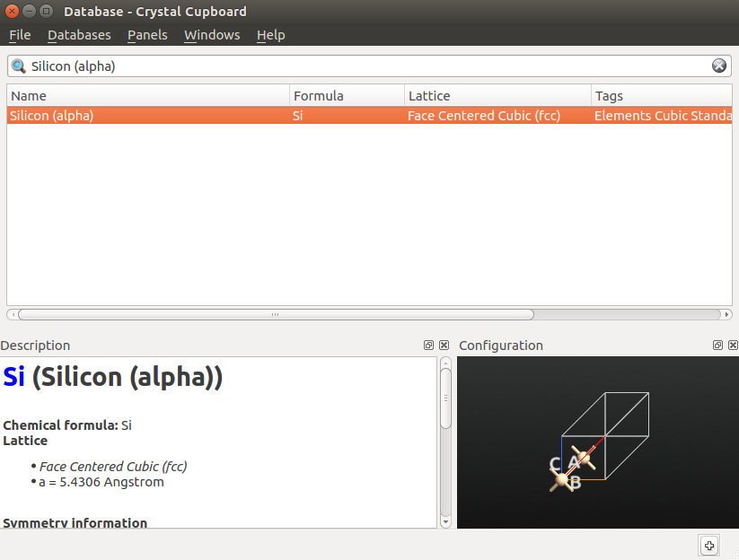
Open the
 Builder and select
to access QuantumATK’s database of compounds.
Builder and select
to access QuantumATK’s database of compounds.Search for “Silicon (alpha)” and add it to the stash by clicking the
 icon in the lower right corner.
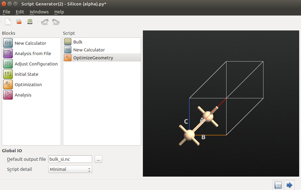
Send the configuration to the
 Script Generator (use the
  icon for this), and add the following blocks to the script:
New Calculator
OptimizeGeometry
Then change the default output file to bulk_si.hdf5.
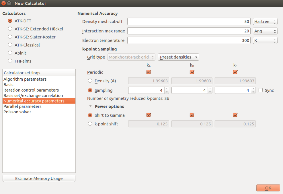
Next, we will choose calculator settings that are optimized for speed rather than accuracy, in order to show the functionality of the AKMC algorithm with DFT. Always check the accuracy of your settings when you want publication-quality data.
New Calculator
Basis set: SingleZetaPolarized
Exchange-Correlation: GGA.PBES to use the PBEsol functional.
k-point sampling: 4x4x4 and make sure it is shifted to gamma by ticking the three boxes found by ticking More options. This is a very low k-point density, but equivalent to the sampling we will use during the AKMC, where we will use only the gamma point to speed things up.
Set the mesh cutoff to 50 Hartree.
OptimizeGeometry
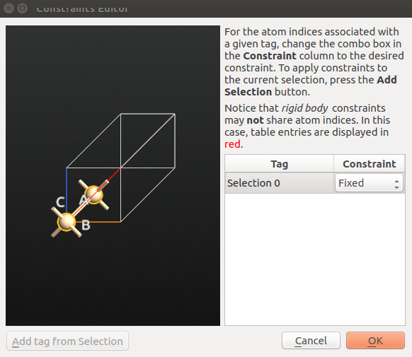
Untick Constrain Lattice Vectors.
Keep the fractional coordinates of Si atoms fixed:
open Atomic Constraint Editor and select one Si atom;
hold down
Ctrlwhile selecting the other atom and click Add tag from Selection.choose Fixed under Constraint and click “OK”.
Leave everything else at default in the OptimizeGeometry block and send the script to the
 Job Manager to run the script. The calculation will take a few minutes.
Build the B-doped Si crystal structure
Once the calculation is finished, you can find the optimized Si bulk structure on the LabFloor.
Select the optimized geometry and drop it on the
Builder.Make the cell cubic by clicking on , then click on Conventional and then Transform. Note how the number of atoms has increased to 8.
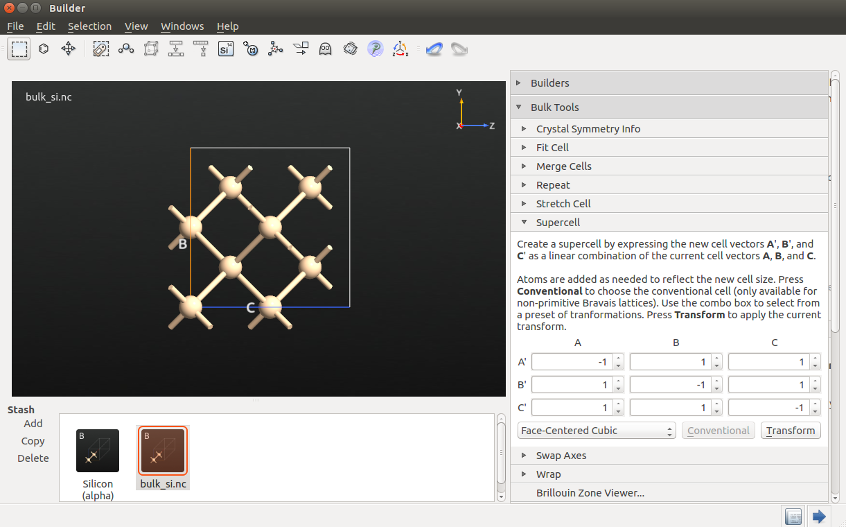
To make the 64 atom cell, click and increase A, B and C to 2 before clicking Apply.
Select the Si atom you would like to replace with B, e.g. atom number 8, close to the origin at [0.125, 0.125, 0.125] in fractional coordinates.
Click the
 Periodic Table plugin and select B in the periodic table.
Setup the script
Send the structure to the Script Generator, change the default output file to sib-optimized.hdf5, and add the following blocks to the script:
- New Calculator
- OptimizeGeometry
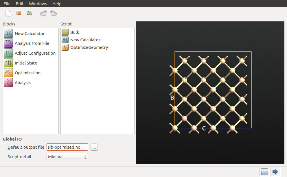
Next, choose the following settings for the respective blocks.
New Calculator:
k-points sampling: 1x1x1, sampling only the gamma point;
basis set: SingleZetaPolarized for Silicon and DoubleZetaPolarized for Boron;
apply the same settings as before for everything else.
OptimizeGeometry: change the convergence criterion to 0.01 eV/Å, and keep the default values for everything else.
Send the script to the Job Manager and run the script.
When the job has finished after about 10 minutes, depending on hardware, we are ready to do the actual AKMC simulation.
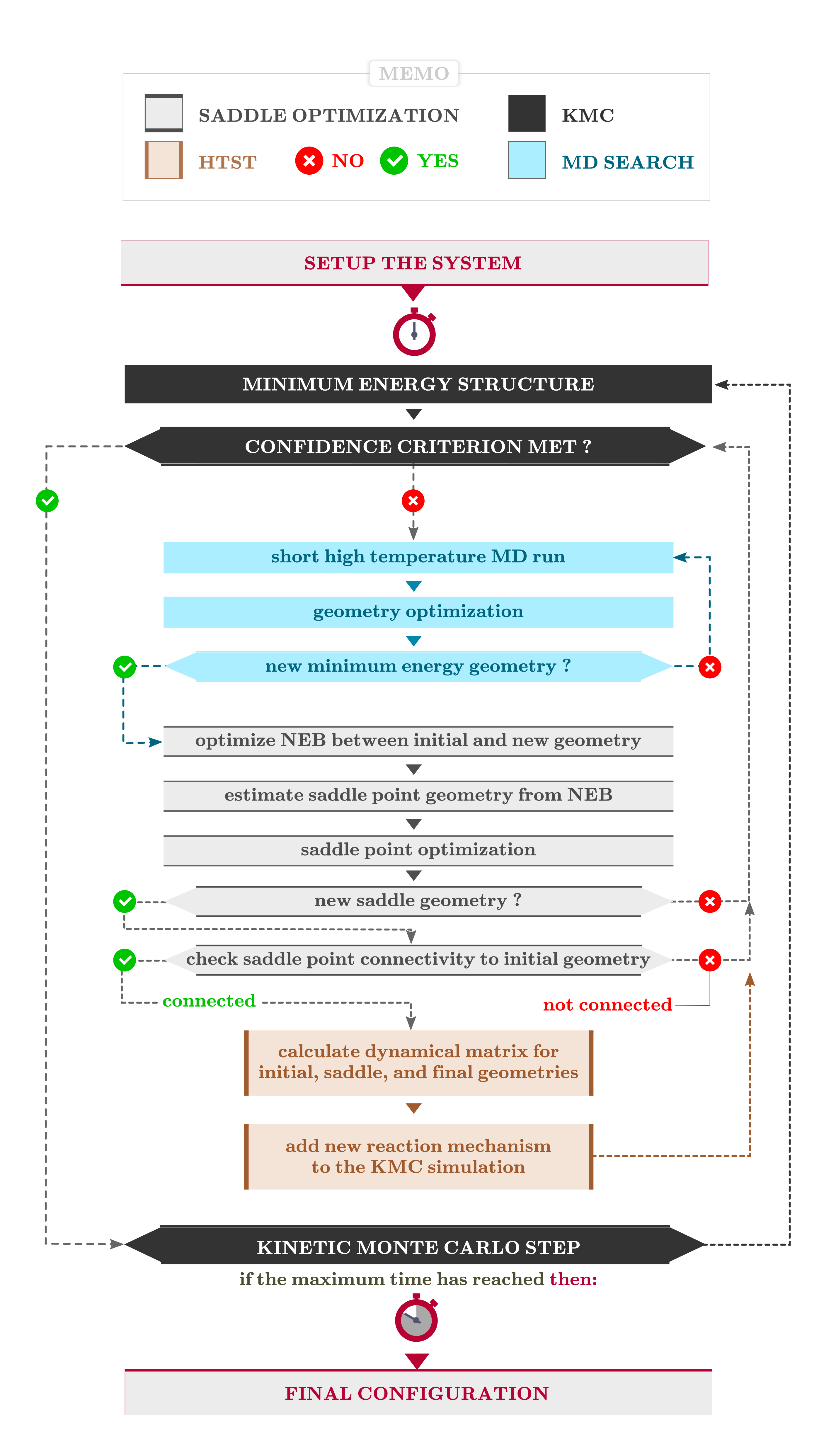
Running the AKMC simulation
Setting up the AKMC calculation requires using only a few lines of Python scripting,
and has been prepared in the script sib-with-akmc.py. The different parts of the script will be explained below.
Download the script, and make sure the file name in the beginning points at the file with your optimized  BulkConfiguration.
Note
Support for setting up an AKMC calculation using the Script Generator is planned for QuantumATK 2017.
Details of the script
First, we change the logging behavior of QuantumATK to the verbosity mode MinimalLog, which will greatly reduce the information in the log file for each SCF cycle. This will improve readability of the log files from the AKMC simulation, while leaving essential SCF information available. The optimized configuration is then loaded from the saved .hdf5-file.
setVerbosity(MinimalLog)

# -------------------------------------------------------------
# Bulk Configuration
# -------------------------------------------------------------

# Read in configuration
bulk_configuration = nlread('../sib-optimized.nc', BulkConfiguration)[-1]
See also
For more information on how to tune the verbosity of QuantumATK logging output, see the Reference Manual entry on setVerbosity(). In particular, the options “CALCULATOR_UPDATE=False” and “PROGRESS_BARS=False” could be relevant here; they remove all the SCF information and progress bars from the output, respectively.
We then proceed to set up a calculator that is identical
to the one used for structural relaxation, except for the addition of the ParallelParameters functionality, which is used to ensure that just one
process will be used for each AKMC saddle search. For a bigger system, it might make sense to use more than one process per saddle
search, but the optimal distribution depends on the setup and queuing rules of your supercomputer.
# -------------------------------------------------------------
# Calculator
# -------------------------------------------------------------
#----------------------------------------
# Basis Set
#----------------------------------------
basis_set = [
    GGABasis.Boron_DoubleZetaPolarized,
    GGABasis.Silicon_SingleZetaPolarized,
    ]

#----------------------------------------
# Exchange-Correlation
#----------------------------------------
exchange_correlation = GGA.PBES

k_point_sampling = MonkhorstPackGrid(
    na=1,
    nb=1,
    nc=1,
    shift_to_gamma=[True, True, True],
    )
numerical_accuracy_parameters = NumericalAccuracyParameters(
    k_point_sampling=k_point_sampling,
    density_mesh_cutoff=50.0*Hartree
    )

parallel_parameters = ParallelParameters(
    processes_per_saddle_search=1,
    )

calculator = LCAOCalculator(
    basis_set=basis_set,
    exchange_correlation=exchange_correlation,
    numerical_accuracy_parameters=numerical_accuracy_parameters,
    parallel_parameters=parallel_parameters,
    )

bulk_configuration.setCalculator(calculator)
nlprint(bulk_configuration)
bulk_configuration.update()
The final part of the script is the actual AKMC simulation. First, there are two blocks which check if a previous AKMC simulation has already been run, and reuse that information if possible, or initialize new objects if no previous results are present.
# --------------------------------------------------------------
# AKMC
# --------------------------------------------------------------

# Reusing existing MarkovChain object if it already exists, otherwise a new one is created
if os.path.isfile('akmc_markov_chain.nc'):
    markov_chain = nlread('akmc_markov_chain.nc')[0]
else:
    markov_chain = MarkovChain(bulk_configuration, TotalEnergy(bulk_configuration).evaluate())

# Reusing existing KMC object if it already exists, otherwise a new one is created
if os.path.isfile('akmc_kmc.nc'):
    kmc = nlread('akmc_kmc.nc')[0]
else:
    kmc = None
Next comes SaddleSearchParameters, where we restrict NEB calculations to no more than 5 images. For this system, we expect fairly simple reactions, which will be well-described with 5 images or less. For more complicated systems, more than 5 images per NEB might be needed. This is not a very expensive part of the overall calculation, but we need to optimize for speed when using DFT.
# Modify the default maximum number of NEB images to 5.
saddle_search_parameters = SaddleSearchParameters(max_neb_images=5)
Finally the AKMC calculation is set up, including the SaddleSearchParameters object, and then started in the final line. For solid state systems it is often a good approximation to assume the prefactor, which is very expensive to calculate. In this case we use a value of 1013 s-1, which should be appropriate for this system. As AKMC is a stochastic method, it is important to do enough saddle searches to ensure the reaction space is adequately sampled. This is also why this script is designed to make additional runs straightforward to do.
# Setup the AKMC simulation.
akmc = AdaptiveKineticMonteCarlo(markov_chain,
                                 calculator=calculator,
                                 kmc_temperature=300*Kelvin,
                                 md_temperature=3000*Kelvin,
                                 saddle_search_parameters=saddle_search_parameters,
                                 constraints=[15],
				 kmc=kmc,
                                 confidence=0.99,
				 assumed_prefactor=1e13/Second,
                                 write_searches=False,
                                 write_kmc=True,
                                 write_markov_chain=True,
                                 write_log=True)

# Run 200 saddle searches.
akmc.run(200)
Warning
In AKMC calculations, you must constrain at least one atom to avoid drift of the system during the high-temperature MD. However, this will introduce a slight error in the potential energy surface (PES) close to the constrained atom(s), so the constraint(s) should in general be applied as far as possible from where you expect transitions to happen. In this case the constraint is chosen to be an atom exactly half a supercell away from the B atom in all directions, to minimize the impact on any reactions involving B.
Note
For further information on the parameters in the AKMC calculation, see for example the tutorial: Modeling Vacancy Diffusion in Si0.5 Ge0.5 with AKMC . In the present tutorial we focus on those features which need special attention when a DFT calculator is used.
Running the AKMC job
The script needs to run on a supercomputer, as it takes up to two full days per saddle search. In this case we run 2x50 hours on 3 nodes, for a total of 48 cores.
Attention
If you modify the parallelization options to better fit your system and the architecture of your favorite supercomputer, remember to leave one process for the AKMC algorithm itself. If you have N available CPU cores, only N-1 cores are available for saddle searches.
Analyzing the results
The script generates the following output files:
One log-file for each saddle search:
saddle_search_*_*.log
The central log-file for the AKMC algorithm:
akmc_log.hdf5
A file containing the Markov Chain object:
akmc_markov_chain.hdf5
If any KMC steps have been taken by the algorithm: A file containing the Kinetic Monte Carlo object:
akmc_kmc.hdf5
A file containing everything sent to std out:
sib-with-akmc.log
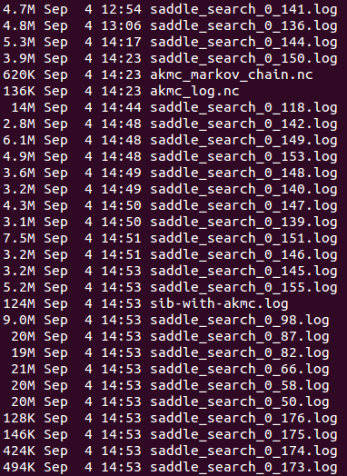
In this case, no KMC steps have been taken, so there is no file named akmc_kmc.hdf5. This is also why all the saddle search files have a 0 as the first number; they have all been started from the original initial state. Many of the saddle search files have the same time-stamp, as they have been killed by the queuing system on the cluster.
Inspecting the AKMC log-file
The AKMC log file can be most easily inspected using Text Representation… in the QuantumATK Panel bar. This will bring up the following window:
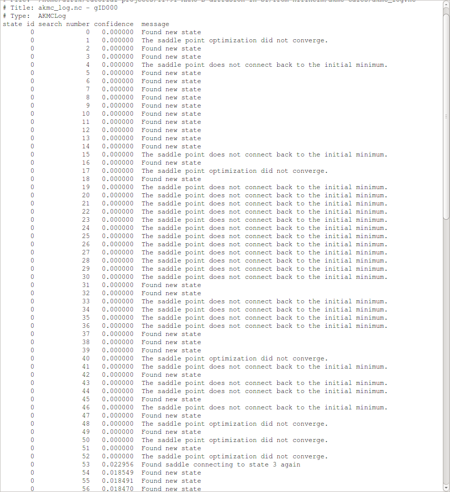
This shows information about each completed saddle search.
“state id” is the id number of the state, which the saddle searches are originating from – in this case state 0, which is the original initial state.
“search number” is the id number of the saddle search, corresponding to the second number in the name of the log files.
“confidence” is the confidence, on a scale from 0 to 1, that the current initial state has been adequately sampled.
“message” is a short message describing the result of the saddle search.
We see that many saddle searches find new states and that about as many find saddle points which are not connected to the initial state. The former indicates that there are many saddle points with similar barriers, while the latter indicates that the potential energy surface (PES) is somewhat complicated. The confidence remains low because many searches discover new states, while only one search finds an already known state. This indicates that there are many relevant states, and the algorithm thus requires much more data before the PES has been adequately sampled around our original initial state and the first KMC step can be performed.
Inspecting the Markov Chain
The Markov Chain is a list of all the discovered states and the connections between them. It can be visualized using the Markov Chain analyzer plugin in the QuantumATK panel bar. In this case, all the connections originate in the original initial state (state 0). You can view all the connections for a different state by changing State to a value other than 0. You can also change the Temperature to see how the rates change. In this case the rates are all extremely small at 300 K, as the barriers are quite high. However, due to the exponential dependence of the rate on 1/T, doubling the temperature to 600 K increases the rates by about 16 orders of magnitude.
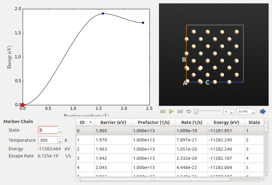
Validating the assumed prefactor
We will now verify that the assumed prefactor used in the AKMC calculations is reasonable. We select the transition between states 0 and 17, as it has the lowest barrier and involves atoms close to the B atom.
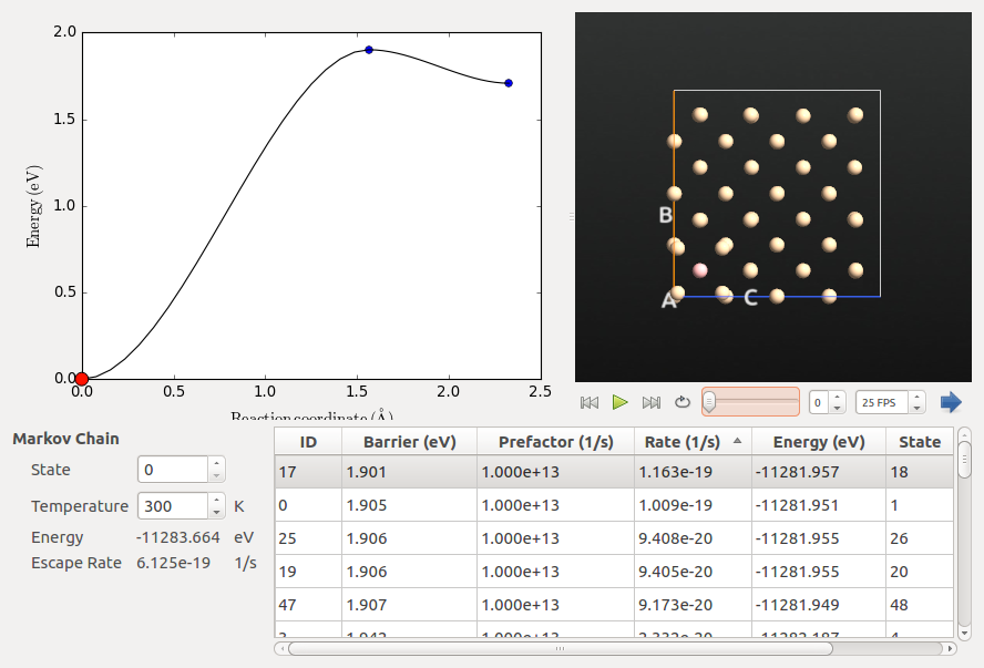
Tip
You can sort the states by each of the columns. In this case, we sorted by barrier to identify the states with the lowest barrier. They also have the highest rates as the prefactor is identical for all transitions.
The procedure for this calculation is as follows:
Extract the initial, saddle and final states from the Markov Chain, and optimize their geometry.
Create a NEB configuration with more images and optimize it, first without and then with climbing image.
Do the actual prefactor calculation using
HTSTEvent.
The first point is covered in the script: extract-neb-from-markov-chain.py. The Markov Chain object stores the final states and saddle point states for all the discovered transitions between the known states. These configurations can then be extracted as shown in the first lines of code below, for the initial and final states. Afterwards, we define a calculator identical to the one used in the AKMC simulation and optimize the geometry with a tolerance of 0.01 eV/Å. This is a stricter criterion than the default in OptimizeGeometry, but identical to the default in the AKMC simulation, which is selected to ensure convergence of the prefactor calculation. For some systems it might be needed to converge even more tightly.
markov_chain = nlread('akmc_markov_chain.nc')[0]

initial_state_id = 0
final_state_id = 17

initial_conf = markov_chain.getStateConfiguration(initial_state_id)
final_conf = markov_chain.getStateConfiguration(final_state_id)
extract-neb-from-markov-chain.py
In the next script, optimize-neb-from-markov-chain.py, we create a NEB configuration based on the minimized initial and final configurations, plus the saddle configuration as extracted from the Markov Chain.
markov_chain = nlread('akmc_markov_chain.nc')[0]

initial_conf = nlread('initial_conf.nc',BulkConfiguration)[-1]
final_conf = nlread('final_conf.nc',BulkConfiguration)[-1]

initial_state_id = 0
final_state_id = 17

# Make the NEB configuration

saddle_conf = markov_chain.getSaddleConfiguration(initial_state_id, final_state_id)

configuration_list = [initial_conf, saddle_conf, final_conf]

neb_configuration = NudgedElasticBand(configuration_list, image_distance=1.0*Angstrom, generate_images=True, wrap_pbc=True)

nlsave('neb-configuration.nc',neb_configuration)
Then we define a calculator identical to the one used in the AKMC simulation (not shown here), and proceed to optimize the NEB; this is done with a regular optimization first, and then an additional one with climbing image turned on. This optimization can take several hours, even on a multi-core machine.
neb_configuration.setCalculator(calculator)

optimized_neb_configuration = OptimizeNudgedElasticBand(
        neb_configuration,
        max_forces=0.01*eV/Ang)

nlsave('optimized-neb-configuration.nc',optimized_neb_configuration)

ci_optimized_neb_configuration = OptimizeNudgedElasticBand(
        optimized_neb_configuration,
	climbing_image=True,
        max_forces=0.01*eV/Ang)

nlsave('ci-optimized-neb-configuration.nc',ci_optimized_neb_configuration)
optimize-neb-from-markov-chain.py
Note
You can also do the NEB optimization with climbing image turned on from the beginning, but this is a less stable approach and can lead to convergence problems. Doing it in two steps, as we do here, is slightly slower, but will be much more likely to converge without issues.
Finally, we calculate the prefactor with a simple script using HTSTEvent, reading in the fully optimized NEB configuration.
neb_configuration = nlread('ci-optimized-neb-configuration.nc',NudgedElasticBand)[-1]

# -------------------------------------------------------------
# HTST Event
# -------------------------------------------------------------
htst_event = HTSTEvent(
    neb_configuration,
    finite_difference_method=Central,
    minimum_displacement=0.05*Angstrom,
    )
nlsave('htst-event.nc', htst_event)
nlprint(htst_event)
This script requires approximately 600 energy and force calculations and ran for about 2.5 hours on an 8-core node. When it has finished, the results are found at the end of the log-file containing the std output:
+------------------------------------------------------------------------------+
|                                                                              |
| HTST Event Information                                                       |
|                                                                              |
+------------------------------------------------------------------------------+
|    Reactant Energy: -11283.6643027 eV                                        |
|    Saddle   Energy: -11281.7203394 eV                                        |
|    Product  Energy: -11282.1925809 eV                                        |
|   Forward  Barrier:      1.9439633 eV                                        |
|   Backward Barrier:      0.4722415 eV                                        |
| Forward  Prefactor:      1.792e+14 1/s                                       |
| Backward Prefactor:      6.939e+13 1/s                                       |
+------------------------------------------------------------------------------+
We see that the forward prefactor is a little more than an order of magnitude larger than the estimated value of 1013 s-1, while the backward prefactor is a little less than an order of magnitude off. This validates our assumed prefactor, as this deviation from the assumption is much smaller than the many orders of magnitude the rate can vary due to the exponential dependence on the barrier.
Conclusions
The AKMC simulations indicate that atomic boron in bulk silicon is very stable in a substitutional lattice site, and effectively immobile at temperatures close to room temperature. A reaction rate prefactor of 1013 s-1 per second was assumed and later verified.