Occupation Methods
This document explains and compares the different occupation methods available in ATK. We suggest these guidelines for choosing the occupation method, depending on the system of interest:
Systems with a band-gap (semiconductors, insulators, molecules): Use either Fermi-Dirac or Gaussian smearing with a low broadening, e.g. around 0.01 eV.
Metals : Use either Methfessel-Paxton or cold smearing with as large a broadening as possible as long as the entropy contribution to the free energy remains small.
If you are interested in understanding the rationale behind these suggestions, you can read the Background and the Comparison of smearing methods sections below.
Note
The smearing width of the Fermi-Dirac distribution is roughly a factor of two larger than for the other functions. Therefore, in order to obtain the same \(\mathbf{k}\)-point convergence using one of these methods as obtained with the Fermi-Dirac method one has to use a broadening of twice the size.
Background
Introduction to smearing methods
In ATK-DFT and ATK-SE the central object is the electron density \(n(\mathbf{r})\) which is calculated from the Kohn-Sham eigenvectors \(\psi_n(\mathbf{r})\) by the expression
where the index \(i\) runs over all states and \(f_i\) are the occupation numbers. The latter can be either 1 if the given state is occupied or 0 if the state is unoccupied. In periodic systems such as bulk materials or surfaces, the sum over states involves an integration over the Brillouin zone (BZ) of the system:
In practice this integration is carried out numerically by summing over a finite set of \(\mathbf{k}\)-points. For gapped systems the density and derived quantities, like the total energy, converge quickly with the number of \(\mathbf{k}\)-points used in the integration. However, for metals the bands crossing the Fermi level are only partially occupied, and a discontinuity exists at the Fermi surface, where the occupancies suddenly jump from 1 to 0. In this case, one will often need a prohibitively large amount of \(\mathbf{k}\)-points in order to make calculations converge.
The number of \(\mathbf{k}\)-points needed to make the calculations converge can be drastically reduced by replacing the integer occupation numbers \(f_{i\mathbf{k}}\) by a function that varies smoothly from 1 to 0 close to the Fermi level. The most natural choice is the Fermi-Dirac distribution,
where \(\epsilon_{i\mathbf{k}}\) is the energy, \(\mu\) is the chemical potential and \(\sigma=k_\text{B}T\) is the broadening.
Fig. 216 shows the convergence of the total energy of bulk Aluminum, a typical simple metal.
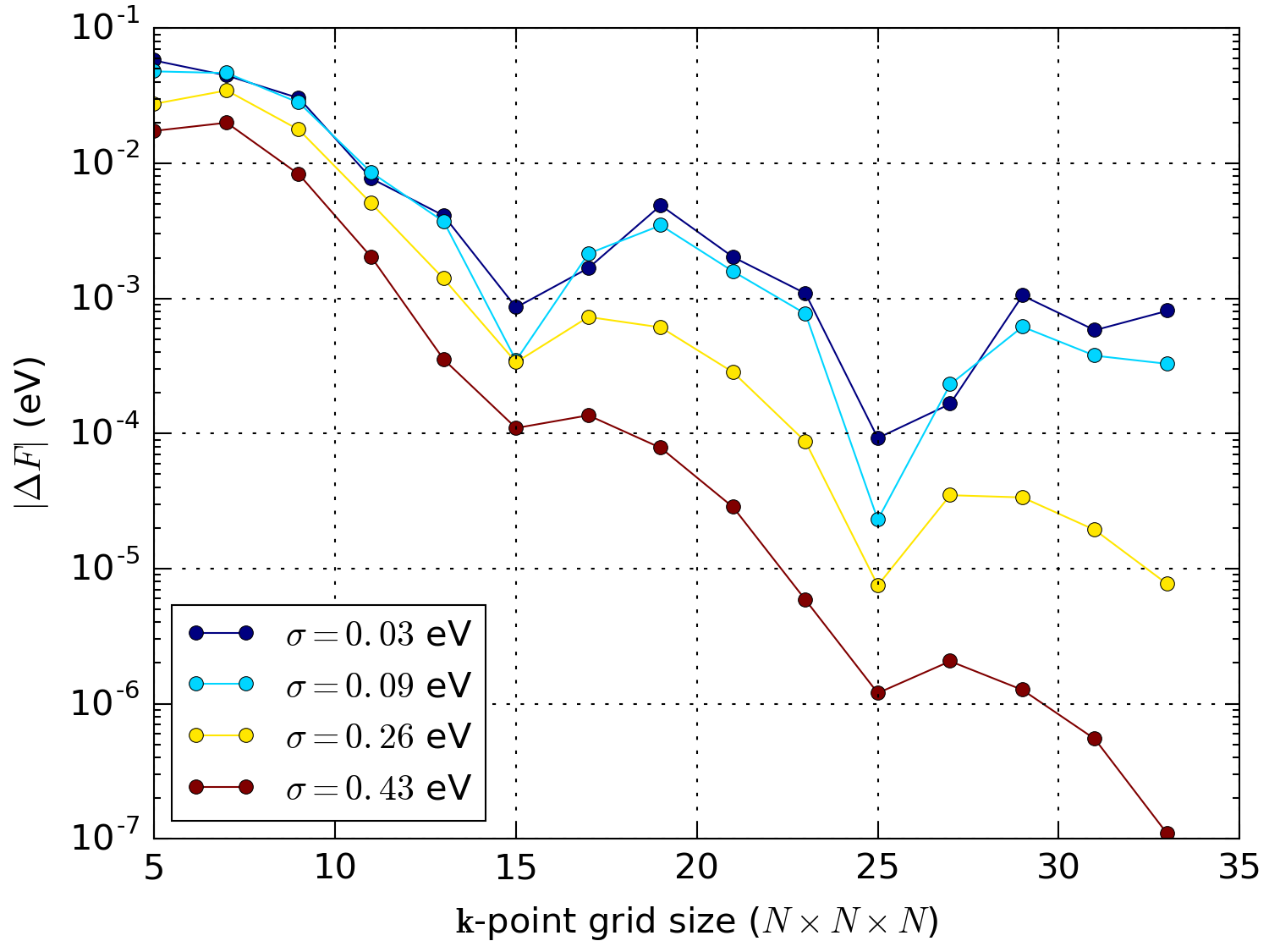
Fig. 216 Convergence of the free energy of bulk Aluminum with respect to the k-point sampling using the Fermi-Dirac occupation function with different broadenings. The free energy difference, \(\Delta F\), is calculated as the difference between the calculation at the given \(\mathbf{k}\)-point sampling and one at \(35\times 35\times 35\).
We see that using \(\sigma\) = 0.03 eV one needs a \(25\times 25\times 25\) \(\mathbf{k}\)-point sampling grid (a total of 15625 \(\mathbf{k}\)-points) in order to converge the total energy within 1 meV, whereas using \(\sigma\) = 0.43 eV the total energy is converged to within 1 meV using only a \(13\times 13\times 13\) grid (a total of 2197 \(\mathbf{k}\)-points). This results in a calculation which roughly is a factor of 7 faster.
Free energy functional
When introducing the Fermi-Dirac distribution one effectively considers an equivalent system of non-interacting electrons at a temperature \(T\). This also means that the variational internal energy functional \(E[n]\) that is minimized is replaced by the free energy functional [1]
where \(S\) is the electronic entropy. All derived quantities such as the density, total energy, forces, etc., will therefore depend on the electron temperature \(T\). If one is actually interested in simulating a system at finite temperature, then the free energy is the relevant functional. If that is not the case, the zero-temperature internal energy \(E(\sigma=0)\) can still be extrapolated from the free energy \(F(\sigma)\), due to the quadratic dependence (to the lowest order) of both \(E(\sigma)\) and \(F(\sigma)\) on \(\sigma\) by the formula [2]
Fig. 217 shows that, for all the values of the
broadening \(\sigma\) considered, the value of the energy extrapolated to
\(\sigma \to 0\) is basically spot on the actual value. Using this
extrapolation method it is thus possible to do calculations with very high
broadenings, necessary to converge metallic systems, with a reasonable number
of \(\mathbf{k}\)-points and still get an accurate ground state energy. The
extrapolated energy is by default shown in the output when doing a total energy
calculation using QuantumATK. In order to get the value using QuantumATK see
TotalEnergy.
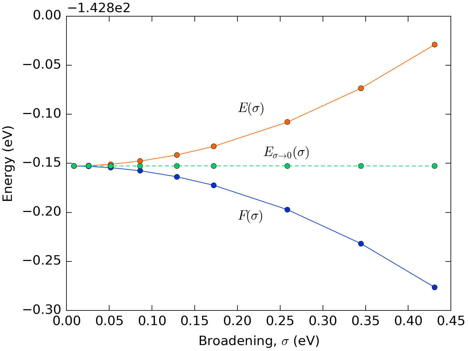
Fig. 217 Total free and internal energy of bulk aluminum as a function of the broadening of the Fermi-Dirac distribution. Calculated with a \(35\times 35\times 35\) \(\mathbf{k}\)-point sampling.
Unfortunately a similar extrapolation method does not exist for forces and stress. Thus these properties will be those that correspond to the free energy and will be directly dependent on the chosen broadening. In order to minimize the errors introduced by the broadening, alternative occupation functions for which the entropic contribution to the free energy is smaller than for the Fermi-Dirac distribution have been developed.
The different occupation functions are introduced on the basis of considering the density of states given by the expression
Since the \(\mathbf{k}\)-point integration is in practice carried out as a sum over a finite number of points, one has to replace the \(\delta\)-function by a smeared function \(\tilde{\delta}(x)\), whose width will be determined by a broadening \(\sigma\). With a choice of smearing function the occupation function is given by
where \(\mu\) is the Fermi level. Even without directly introducing temperature, one can then show that the functional that has to be minimized is the generalized free energy [3][4]. The generalized temperature is given by the broadening \(\sigma\) and smearing method also directly determines the expression for the generalized entropy.
Comparison of smearing methods
In ATK four different smearing methods are available:
Fermi-Dirac distribution (
FermiDirac)Gaussian smearing (
GaussianSmearing) [5]Methfessel-Paxton smearing (
MethfesselPaxton) [6]Cold smearing (
ColdSmearing) [7]
Warning
While the broadening parameter of the Fermi-Dirac distribution has a real physical meaning and can actually be associated with an electronic temperature, this is not true for the other smearing methods, for which the broadening is simply a parameter without a well defined physical meaning!
Fig. 218 shows plots of the smeared \(\delta\)-functions and occupation functions for the different methods.
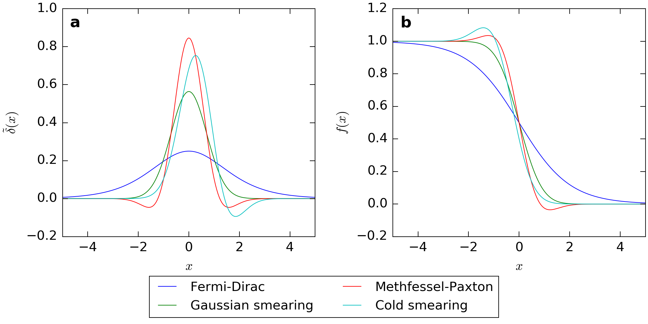
Fig. 218 (a) Plots of the different smeared delta functions, \(\tilde{\delta}(x)\), and (b) their corresponding occupation functions \(f(x)\), shown as functions of \(x = \frac{\epsilon - \mu}{\sigma}\).
From the figure we note a few things:
The width of the Fermi-Dirac smearing function is larger than all the others. The ratio of the full width at half maximum between the Fermi-Dirac and the Gaussian smeared \(\delta\)-function is
\[\alpha = \frac{\text{FWHM}(\text{Fermi-Dirac})}{\text{FWHM}(\text{Gaussian})} = \frac{2 \cosh^{-1}(\sqrt{2})}{\sqrt{\ln(2)}} \approx 2.117.\]This means that in order to get similar \(\mathbf{k}\)-point convergence as for the Fermi-Dirac method one has to use a broadening which is a factor of ~2 larger when using one of the other methods.
The Methfessel-Paxton function is special in that the occupations may take unphysical negative values and values larger than one. For insulators and semiconductors as well as too coarsely sampled metals this may lead to negative density of states and a negative density, which may cause computational problems.
The cold smearing function is asymmetric but does not attain negative values and problems with negative density are therefore avoided.
From Fig. 219 it can be seen that for the Methfessel-Paxton and cold smearing the free energy, \(F(\sigma)\), hardly varies with \(\sigma\). In fact it can be shown that for these two methods \(F(\sigma)\) only has 3rd and higher order dependences on \(\sigma\).
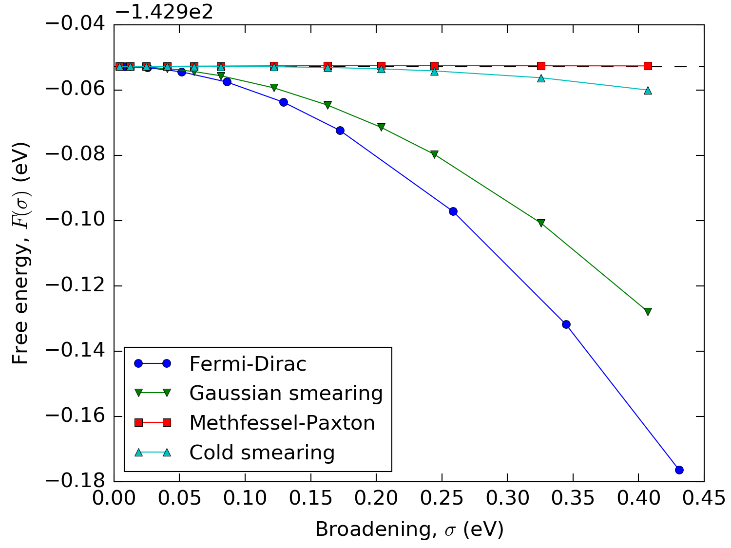
Fig. 219 Free energy of bulk Aluminum calculated with different occupation methods and values of the broadening using a \(\mathbf{k}\)-point sampling of \(35\times 35\times 35\). In order to keep the different methods comparable, the broadening has been multiplied by 2.117 for all but the Fermi-Dirac distribution.
The low \(\sigma\) dependence on the free energy for Methfessel-Paxton and cold smearing should be carried over in derived quantities like forces and stress. This is indeed the case as illustrated in Fig. 220, which shows the force on the uppermost atom in a 6 layer Aluminum 111 slab as a function of the used broadening.
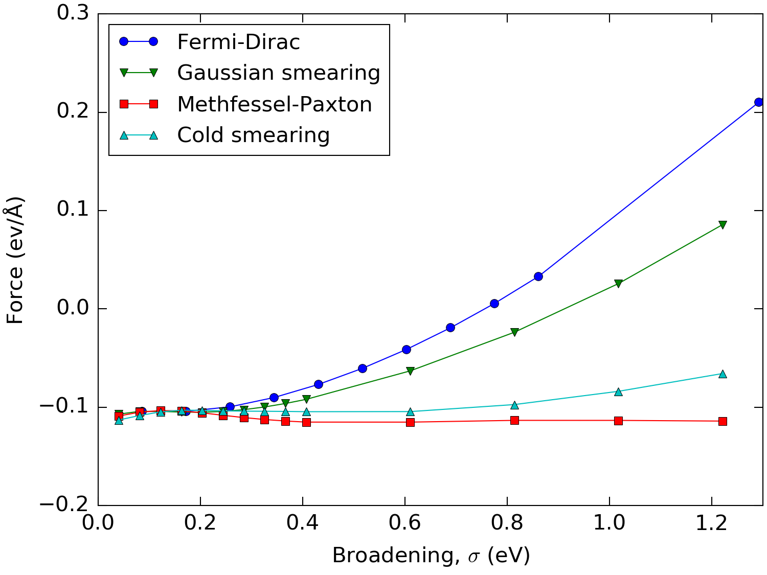
Fig. 220 Force on the outermost atom in a 6 layer Aluminum 111 slab as a function of the broadening using the different occupation methods. In order to keep the different methods comparable, the broadening has been multiplied by 2.117 for all but the Fermi-Dirac distribution.
We see that for small values of the broadening the outer layers seek to contract, whereas this effect is reversed for the Fermi-Dirac distribution at a broadening of about 0.75 eV due to the introduced electron gas pressure. For Methfessel-Paxton and cold smearing the error is neglible for a large range of values for the broadening. This means that one can efficiently calculate accurate forces (for example, during structural optimizations, ab-initio molecular dyanmics and phonons calculations) for metals using sizeable broadenings and relatively low \(\mathbf{k}\)-point samplings.