Relativistic effects in bulk gold
Gold is one of the more heavy transition metals, and the electronic structure of bulk gold is therefore significantly affected by relativistic effects, including spin-orbit coupling (SOC).
Relativistic ab initio band structure calculations for gold were first reported in the early 1970s, see e.g. Refs. [1], [2], and [3]. Those studies, and later ones, found that relativistic effects cause a significant reorganization of the electronic energy bands in gold. In particular, inclusion of relativistic effects removes a large part of the band crossings in the deeper valence bands found in standard calculations. In this tutorial, you will demonstrate this using ATK-DFT for standard scalar-relativistic (GGA) and relativistic (SOGGA) calculations of the gold band structure.
GGA band structure
Use the QuantumATK Builder  to create the gold bulk configuration.
This is most easily done using the
tool. Keep the gold lattice constant at the experimental value (4.078 Å).
to create the gold bulk configuration.
This is most easily done using the
tool. Keep the gold lattice constant at the experimental value (4.078 Å).
Then transfer the configuration to the Script Generator  and set up a standard GGA-PBE band structure calculation using an OMX
pseudopotential.
and set up a standard GGA-PBE band structure calculation using an OMX
pseudopotential.
First, add a New Calculator  block and a
Bandstructure
block and a
Bandstructure  analysis block, and set
 gold_gga.nc
as the output file.

Edit the New Calculator settings:
In the Basis set/exchange correlation panel, choose the GGA-PBE exchange-correlation functional and the OMX pseudopotential with a Medium accuracy basis set.
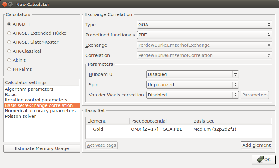
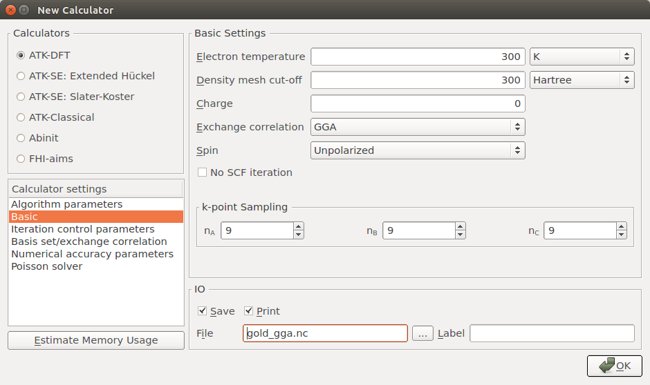
In the Basic panel, set the Density mesh-cutoff to 300 Hartree and increase the k-point Sampling to 9x9x9.
Open the Bandstructure block and edit it:
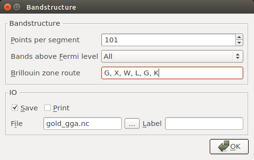
Increase Points per segment to 101 in order to finely sample the band structure between each high-symmetry point, and trim the default Brillouin zone route such that it reads “G, X, W, L, G, K”.
Save the script as gold_gga.py and run it. You can use the Job
Manager  for this. It should take around a minute if
executed on a single processor.
for this. It should take around a minute if
executed on a single processor.
Results
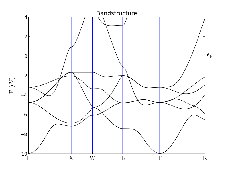
Find the Bandstructure object in the output file on the QuantumATK LabFloor and use the Bandstructure Analyzer to plot it. The results are shown below and are very similar to those reported in Refs. [2] and [3]. Gold is clearly not an insulator, since there are plenty of bands crossing the Fermi level. Also note the frequent band crossing in the deeper valence bands, from ca. -2 to -5 eV below the Fermi energy. As we shall see, most of these crossings disappear in a relativistic calculation including SO interactions.
Spin-orbit GGA band structure
You will here set up and execute a GGA calculation that includes the SOC. This must be done in a noncollinear representation of electron spin, which is computationally more expensive than the GGA calculation and can exhibit poor SCF convergence. You should therefore apply two tricks: a) start the noncollinear calculation from a converged spin-polarized state (SGGA), and b) use a special electron density mixing scheme.
Note
We know that gold is not magnetic, so it may seem a bit silly to do a spin-polarized calculation for gold. After all, the results should not differ from those found in the collinear spin-compensated calculation done in the previous section.
Indeed, they do not, but the converged spin-polarized state offers a much better initial guess for the self-consistent noncollinear+SO state than the spin-compensated state does: Fewer noncollinear SCF steps are required if starting from the spin-polarized state, and computational time is therefore saved.
SGGA initial state
You have two options for setting up a script for the SGGA calculation:
Use the Scripter: Set up the script exactly like in the previous section, but choose “Polarized” for the Spin parameter, remove the Bandstructure analysis object, set the output file to
gold_sgga.nc, and save the new script asgold_sgga.py.Use the Editor: Copy
gold_gga.pytogold_sgga.pyand open the new script in the Editor and edit it a bit.
Set the exchange-correlation to
and edit it a bit.
Set the exchange-correlation to SGGA.PBE, remove the bottom lines that execute the bandstructure calculation, and rename the output file togold_sgga.nc.
In any case, the script should look like this:
# -------------------------------------------------------------
# Bulk Configuration
# -------------------------------------------------------------

# Set up lattice
lattice = FaceCenteredCubic(4.07825*Angstrom)

# Define elements
elements = [Gold]

# Define coordinates
fractional_coordinates = [[ 0.,  0.,  0.]]

# Set up configuration
bulk_configuration = BulkConfiguration(
    bravais_lattice=lattice,
    elements=elements,
    fractional_coordinates=fractional_coordinates
    )

# -------------------------------------------------------------
# Calculator
# -------------------------------------------------------------
#----------------------------------------
# Basis Set
#----------------------------------------

GoldBasis = OpenMXBasisSet(
    element=PeriodicTable.Gold,
    filename="openmx/pao/Au7.0.pao.zip",
    atomic_species="s2p2d2f1",
    pseudopotential=NormConservingPseudoPotential("normconserving/upf2/Au_PBE13.upf.zip"),
    )

basis_set = [
    GoldBasis,
    ]

#----------------------------------------
# Exchange-Correlation
#----------------------------------------
exchange_correlation = SGGA.PBE

numerical_accuracy_parameters = NumericalAccuracyParameters(
    k_point_sampling=(9, 9, 9),
    density_mesh_cutoff=300.0*Hartree,
    )

calculator = LCAOCalculator(
    basis_set=basis_set,
    exchange_correlation=exchange_correlation,
    numerical_accuracy_parameters=numerical_accuracy_parameters,
    )

bulk_configuration.setCalculator(calculator)
nlprint(bulk_configuration)
bulk_configuration.update()
nlsave('gold_sgga.nc', bulk_configuration)
Run the script, it should be very fast. Note that the output file
gold_sgga.nc is generated and that it contains only a single
object;  the gold bulk configuration including the
self-consistent SGGA electronic state, which will be used in the next step.
the gold bulk configuration including the
self-consistent SGGA electronic state, which will be used in the next step.
SOGGA band structure
Use the script below to perform the following work-flow:
Read the
bulk_configurationfrom the filegold_sgga.nc.Get the
calculatorused in the SGGA calculation and modify it slightly; use the SOGGA exchange-correlation and a special mixing scheme for noncollinear calculations.Use the converged SGGA state as initial guess for the SOGGA electron density.
Do the SOGGA ground state calculation followed by band structure analysis.
# -------------------------------------------------------------
# Bulk Configuration
# -------------------------------------------------------------
bulk_configuration = nlread('gold_sgga.nc', BulkConfiguration)[0]

# -------------------------------------------------------------
# Calculator
# -------------------------------------------------------------

# Use the special noncollinear mixing scheme
iteration_control_parameters = IterationControlParameters(
    algorithm=PulayMixer(noncollinear_mixing=True)
    )

# Get the calculator and modify it for spin-orbit GGA
calculator = bulk_configuration.calculator()
calculator = calculator(
    exchange_correlation = SOGGA.PBE,
    iteration_control_parameters = iteration_control_parameters
    )

# Setup the initial state from the GGA calculation
bulk_configuration.setCalculator(
    calculator,
    initial_state = bulk_configuration
    )
nlprint(bulk_configuration)
bulk_configuration.update()
nlsave('gold_sogga.nc', bulk_configuration)

# -------------------------------------------------------------
# Bandstructure
# -------------------------------------------------------------
bandstructure = Bandstructure(
    configuration=bulk_configuration,
    route=['G', 'X', 'W', 'L', 'G', 'K'],
    points_per_segment=101,
    bands_above_fermi_level=All
    )
nlsave('gold_sogga.nc', bandstructure)
Save the script as gold_sogga.py and run the calculation. It should
take roughly 6 minutes to finish if executed in parallel on 4 CPUs.
Results
The plot below shows the band structure obtained from the SOGGA calculation. It follows very closely the literature results in Refs. [2] and [3] and is virtually identical to the SOGGA band structure of gold recently published in Ref. [4]. Note how most of the valence band crossings found in the standard GGA calculation have now been lifted.

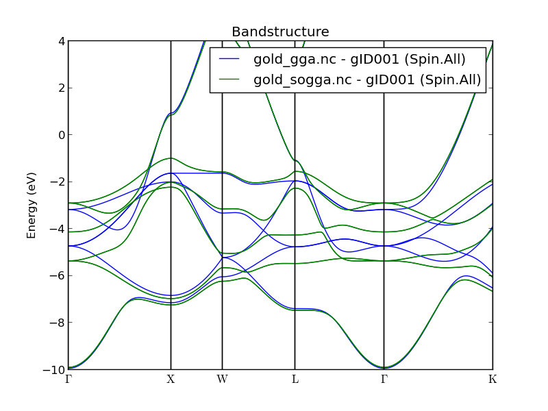
You can also use the Compare Data plugin for a more direct comparison of the two band structures, as illustrated below. Simply highlight both the GGA and the SOGGA bandstructure objects, and click the plugin. It is quite clear that relativistic effects have a significant impact on the gold valence bands. The data illustrated below is essentially identical to that in Figure 6 of Ref. [4].